2. Statistical Basis

Video 1

Hypotheses Multiple testing, ANOVA

2.1. Hypothesis testing and p-value

Questions

Which genes have changes in mean expression level between conditions?

How reliable are this observations (what is your p-value or FDR?)

Here are few slides explaining the concept of hypothesis testing and p-value:

Hypotheses

As an example, let’s do hypothesis testing from the lecture.

mu0 = 3   ## constant to which we compare
m = 2.92  ## experimentally observed mean weight
s = 0.18  ## standard deviation (known in advance)
n = 36    ## number of observations

## standard error (st.dev of mean)
sm = s/sqrt(n) 

## statistics
z = (m-mu0)/sm

## p-value
pnorm(z)

2.2. Parametric test for means (t-test)

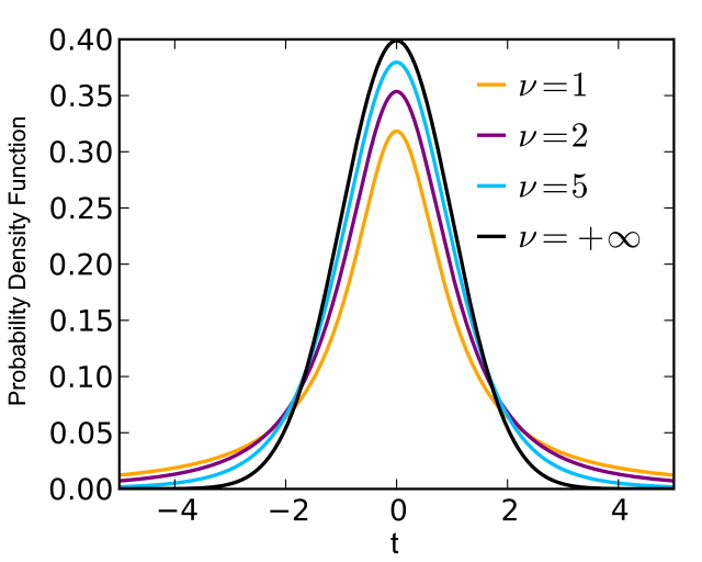
When we work with real data, we need to estimate variance based on experimental observation. This adds additional randomeness => sampling distribution (uncertainty) of mean follows Student (t) distribution.

Student distribution (Wikipedia)

Simple (unpaired) t-test

Let’s test, whether mean weight change differs for male & female mice. Animals in the groups are different, therefore we use unpaired t-test. Corresponding function is t.test()

## load data
Mice=read.table("http://edu.modas.lu/data/txt/mice.txt",header=T,sep="\t",as.is=FALSE)

xm = Mice$Weight.change[Mice$Sex=="m"]
xf = Mice$Weight.change[Mice$Sex=="f"]
t.test(xm,xf)

## 
##  Welch Two Sample t-test
## 
## data:  xm and xf
## t = 3.2067, df = 682.86, p-value = 0.001405
## alternative hypothesis: true difference in means is not equal to 0
## 95 percent confidence interval:
##  0.009873477 0.041059866
## sample estimates:
## mean of x mean of y 
##  1.119401  1.093934

## you can also compare to a constant
## check whether weight change is over 1:
t.test(xm, mu = 1, alternative = c("greater"))

## 
##  One Sample t-test
## 
## data:  xm
## t = 27.334, df = 393, p-value < 2.2e-16
## alternative hypothesis: true mean is greater than 1
## 95 percent confidence interval:
##  1.112199      Inf
## sample estimates:
## mean of x 
##  1.119401

Paired t-test

Example. The systolic blood pressures of n=12 women between the ages of 20 and 35 were measured before and after usage of a newly developed oral contraceptive.

BP=read.table("http://edu.modas.lu/data/txt/bloodpressure.txt",header=T,sep="\t")
str(BP)

## 'data.frame':    12 obs. of  3 variables:
##  $ Subject  : int  1 2 3 4 5 6 7 8 9 10 ...
##  $ BP.before: int  122 126 132 120 142 130 142 137 128 132 ...
##  $ BP.after : int  127 128 140 119 145 130 148 135 129 137 ...

## unpaired
t.test(BP$BP.before,BP$BP.after)

## 
##  Welch Two Sample t-test
## 
## data:  BP$BP.before and BP$BP.after
## t = -0.83189, df = 21.387, p-value = 0.4147
## alternative hypothesis: true difference in means is not equal to 0
## 95 percent confidence interval:
##  -9.034199  3.867532
## sample estimates:
## mean of x mean of y 
##  130.6667  133.2500

## paired
t.test(BP$BP.before,BP$BP.after,paired=T)

## 
##  Paired t-test
## 
## data:  BP$BP.before and BP$BP.after
## t = -2.8976, df = 11, p-value = 0.01451
## alternative hypothesis: true mean difference is not equal to 0
## 95 percent confidence interval:
##  -4.5455745 -0.6210921
## sample estimates:
## mean difference 
##       -2.583333

par(mfcol=c(1,2))
plot(BP$BP.before,BP$BP.after,pch=19,main="Blood pressure")
abline(a=0,b=1,lty=2,col=2)

plot(BP$BP.after-BP$BP.before,pch=19,main="Difference ")
abline(h=0,lty=2,col=2)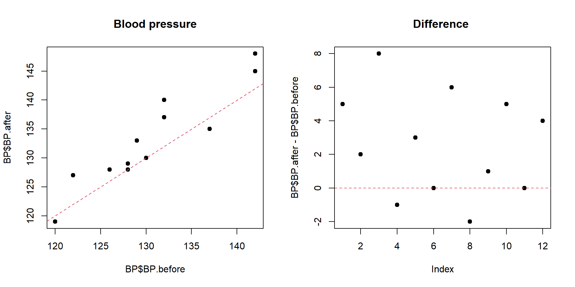

2.3. Non-parametric tests

The Mann–Whitney U test (a.k.a Mann–Whitney–Wilcoxon, Wilcoxon rank-sum, Wilcoxon–Mann–Whitney) is a nonparametric analogue of simple (unpaired) t-test
The Wilcoxon signed-rank test is a non-parametric analogue of a paired t-test

Both tests can be done in R with one command wilcox.test()

## unpaired
wilcox.test(BP$BP.before,BP$BP.after)

## 
##  Wilcoxon rank sum test with continuity correction
## 
## data:  BP$BP.before and BP$BP.after
## W = 59.5, p-value = 0.487
## alternative hypothesis: true location shift is not equal to 0

## paired
wilcox.test(BP$BP.before,BP$BP.after,paired=TRUE)

## 
##  Wilcoxon signed rank test with continuity correction
## 
## data:  BP$BP.before and BP$BP.after
## V = 5, p-value = 0.02465
## alternative hypothesis: true location shift is not equal to 0

2.4. Testing variance

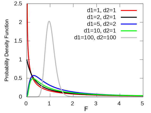
The ratio of sample variances for 2 samples from the same population follows F-distribution (a.k.a. Fisher–Snedecor distribution).

F-distribution (Wikipedia)

You can compare variances of 2 samples using var.test()

Example. A school is selecting a company to provide school bus to its pupils. They would like to choose the most punctual one. The times between bus arrival of two companies were measured and stored in schoolbus dataset. Please test whether the difference is significant with $\alpha = 0.1$.

Bus=read.table("http://edu.modas.lu/data/txt/schoolbus.txt",header=T,sep="\t")
str(Bus)

## 'data.frame':    26 obs. of  2 variables:
##  $ Milbank  : num  35.9 29.9 31.2 16.2 19 15.9 18.8 22.2 19.9 16.4 ...
##  $ Gulf.Park: num  21.6 20.5 23.3 18.8 17.2 7.7 18.6 18.7 20.4 22.4 ...

# see variances
apply(Bus,2,var,na.rm=TRUE)

##   Milbank Gulf.Park 
##  48.02062  19.99996

# test whether they could be the same
var.test(Bus[,1], Bus[,2])

## 
##  F test to compare two variances
## 
## data:  Bus[, 1] and Bus[, 2]
## F = 2.401, num df = 25, denom df = 15, p-value = 0.08105
## alternative hypothesis: true ratio of variances is not equal to 1
## 95 percent confidence interval:
##  0.8927789 5.7887880
## sample estimates:
## ratio of variances 
##           2.401036

2.5. Multiple hypothesis testing

Let’s run a small test described in the lecture: generate a random dataset with 1000 “genes” for 6 “samples”. 3 samples we denote as “A”, 3 - as “B”

library(pheatmap)

ng = 1000  ## n genes
nr = 3     ## n replicates

## random matrix
X = matrix(rnorm(ng*nr*2),nrow=ng, ncol=nr*2)
rownames(X) = paste0("gene",1:ng)
colnames(X) = c(paste0("A",1:nr),paste0("B",1:nr))
pheatmap(X,fontsize_row = 1,cellwidth=20,main="Random expression matrix",scale="row")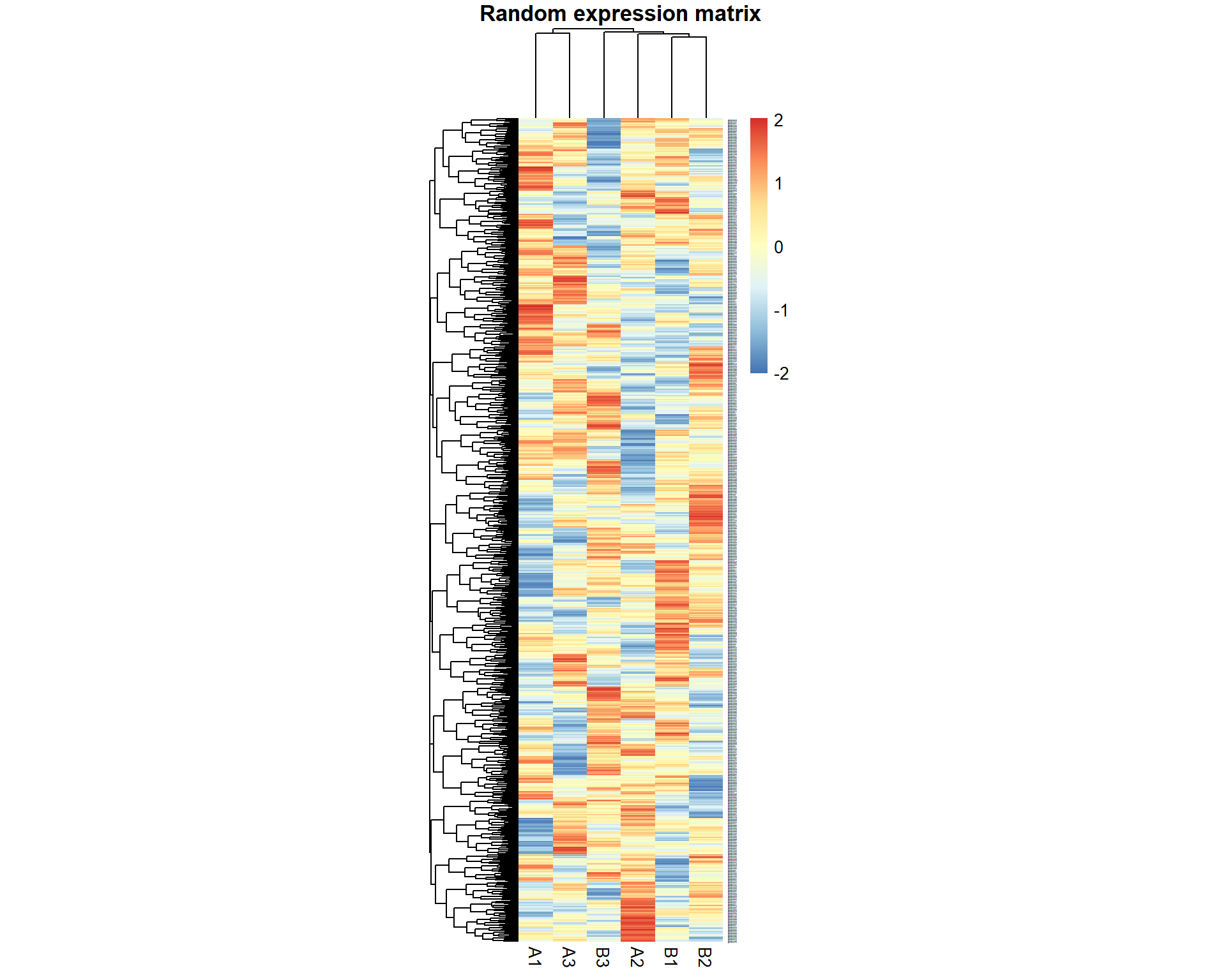

## calculate p-values
pv = double(ng)
names(pv) = rownames(X)
for (i in 1:ng){
  pv[i] = t.test(X[i,1:nr],X[i,(nr+1):(2*nr)])$p.value
}
pheatmap(X[pv<0.05,],cellwidth=20,main="Significant genes by p-value",scale="row")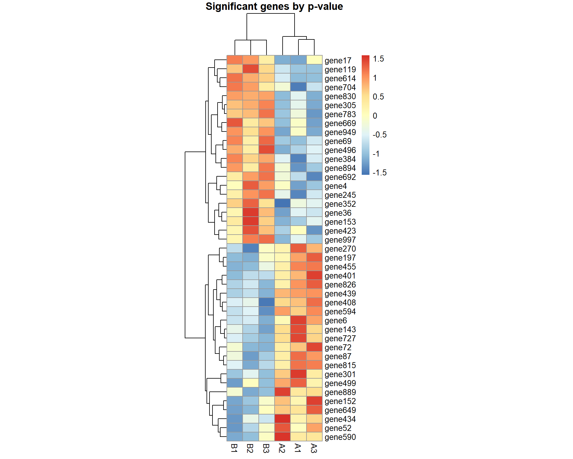

## Significant genes by p-value:
print(names(pv)[pv<0.05])

##  [1] "gene4"   "gene6"   "gene17"  "gene36"  "gene52"  "gene69"  "gene72" 
##  [8] "gene87"  "gene119" "gene143" "gene152" "gene153" "gene197" "gene245"
## [15] "gene270" "gene301" "gene305" "gene352" "gene384" "gene401" "gene408"
## [22] "gene423" "gene434" "gene439" "gene455" "gene496" "gene499" "gene590"
## [29] "gene594" "gene614" "gene649" "gene669" "gene692" "gene704" "gene727"
## [36] "gene783" "gene815" "gene826" "gene830" "gene889" "gene894" "gene949"
## [43] "gene997"

## Correction for multiple testing using Benjamini-Hochberg's FDR and Holm's FWER
fdr = p.adjust(pv,"fdr")
fwer = p.adjust(pv,"holm")

## Significant genes by FDR:
print(names(fdr)[fdr<0.05])

## character(0)

data.frame(PV=pv[pv<0.05],FDR=fdr[pv<0.05],FWER=fwer[pv<0.05])

##                   PV       FDR      FWER
## gene4   0.0470434520 0.9251780 1.0000000
## gene6   0.0413518455 0.9251780 1.0000000
## gene17  0.0377835725 0.9251780 1.0000000
## gene36  0.0344768278 0.9251780 1.0000000
## gene52  0.0482087200 0.9251780 1.0000000
## gene69  0.0196940411 0.9251780 1.0000000
## gene72  0.0268120071 0.9251780 1.0000000
## gene87  0.0159640653 0.9251780 1.0000000
## gene119 0.0123472426 0.9251780 1.0000000
## gene143 0.0134421687 0.9251780 1.0000000
## gene152 0.0392133761 0.9251780 1.0000000
## gene153 0.0247158095 0.9251780 1.0000000
## gene197 0.0359176071 0.9251780 1.0000000
## gene245 0.0190417018 0.9251780 1.0000000
## gene270 0.0463867512 0.9251780 1.0000000
## gene301 0.0267122385 0.9251780 1.0000000
## gene305 0.0071610357 0.9251780 1.0000000
## gene352 0.0379168771 0.9251780 1.0000000
## gene384 0.0175649982 0.9251780 1.0000000
## gene401 0.0318020662 0.9251780 1.0000000
## gene408 0.0237898924 0.9251780 1.0000000
## gene423 0.0499843989 0.9251780 1.0000000
## gene434 0.0427593338 0.9251780 1.0000000
## gene439 0.0007560621 0.6801156 0.7560621
## gene455 0.0136811470 0.9251780 1.0000000
## gene496 0.0188828124 0.9251780 1.0000000
## gene499 0.0386684140 0.9251780 1.0000000
## gene590 0.0470745517 0.9251780 1.0000000
## gene594 0.0099323067 0.9251780 1.0000000
## gene614 0.0013602311 0.6801156 1.0000000
## gene649 0.0331977411 0.9251780 1.0000000
## gene669 0.0286028930 0.9251780 1.0000000
## gene692 0.0240839557 0.9251780 1.0000000
## gene704 0.0300836732 0.9251780 1.0000000
## gene727 0.0137504751 0.9251780 1.0000000
## gene783 0.0158396210 0.9251780 1.0000000
## gene815 0.0146364369 0.9251780 1.0000000
## gene826 0.0232556144 0.9251780 1.0000000
## gene830 0.0136535451 0.9251780 1.0000000
## gene889 0.0273822348 0.9251780 1.0000000
## gene894 0.0203915453 0.9251780 1.0000000
## gene949 0.0300904716 0.9251780 1.0000000
## gene997 0.0214939776 0.9251780 1.0000000

2.6. Analysis of Variance (ANOVA)

Partek’s ANOVA

## load data
Dep = read.table("http://edu.modas.lu/data/txt/depression2.txt",header=T,sep="\t",as.is=FALSE)
str(Dep)

## 'data.frame':    120 obs. of  3 variables:
##  $ Location  : Factor w/ 3 levels "Florida","New York",..: 1 1 1 1 1 1 1 1 1 1 ...
##  $ Health    : Factor w/ 2 levels "bad","good": 2 2 2 2 2 2 2 2 2 2 ...
##  $ Depression: int  3 7 7 3 8 8 8 5 5 2 ...

One-way (one-factor) ANOVA

We start with one-way ANOVA. Let’s consider only healthy respondents in Dep dataset. ANOVA is performed in R: aov(formula, data)

formula - “Values ~ Factor1”, where “Values”, “Factor1” should be replaced by the actual column names in the data frame data

ANOVA tells whether a factor is significant, but tells nothing with treatments (factor levels) are different! Use TukeyHSD() to perform post-hoc analysis and get corrected p-values for the contrasts.

DepGH = Dep[Dep$Health == "good",]

## build 1-factor ANOVA model
res1 = aov(Depression ~  Location, DepGH)
summary(res1)

##             Df Sum Sq Mean Sq F value Pr(>F)   
## Location     2   78.5   39.27   6.773 0.0023 **
## Residuals   57  330.4    5.80                  
## ---
## Signif. codes:  0 '***' 0.001 '**' 0.01 '*' 0.05 '.' 0.1 ' ' 1

TukeyHSD(res1)

##   Tukey multiple comparisons of means
##     95% family-wise confidence level
## 
## Fit: aov(formula = Depression ~ Location, data = DepGH)
## 
## $Location
##                         diff        lwr       upr     p adj
## New York-Florida         2.8  0.9677423 4.6322577 0.0014973
## North Carolina-Florida   1.5 -0.3322577 3.3322577 0.1289579
## North Carolina-New York -1.3 -3.1322577 0.5322577 0.2112612

Two-way (two-factor) ANOVA

For two-way ANOVA the call is similar aov(formula, data). Please note that factor columns in the data frame data should be of class "factor" (newer R version accepts "character"). If factors are "numeric", aov will build regression instead.

formula - “Values ~ Factor1 + Factor2 + Factor1*Factor2”, where “Values”, “Factor1” and “Factor2” should be replaced by the actual column names in the data frame data
Interaction “Factor1*Factor2” can be estimated in case, if you table contains replicates (values measured for the same conditions)

If needed, ANOVA can be followed by TukeyHSD().

## build 2-factor ANOVA model (with interaction)
res2 = aov(Depression ~  Location + Health + Location*Health, Dep)
summary(res2)

##                  Df Sum Sq Mean Sq F value Pr(>F)    
## Location          2   73.8    36.9   4.290  0.016 *  
## Health            1 1748.0  1748.0 203.094 <2e-16 ***
## Location:Health   2   26.1    13.1   1.517  0.224    
## Residuals       114  981.2     8.6                   
## ---
## Signif. codes:  0 '***' 0.001 '**' 0.01 '*' 0.05 '.' 0.1 ' ' 1

TukeyHSD(res2)

##   Tukey multiple comparisons of means
##     95% family-wise confidence level
## 
## Fit: aov(formula = Depression ~ Location + Health + Location * Health, data = Dep)
## 
## $Location
##                           diff        lwr       upr     p adj
## New York-Florida         1.850  0.2921599 3.4078401 0.0155179
## North Carolina-Florida   0.475 -1.0828401 2.0328401 0.7497611
## North Carolina-New York -1.375 -2.9328401 0.1828401 0.0951631
## 
## $Health
##               diff       lwr       upr p adj
## good-bad -7.633333 -8.694414 -6.572252     0
## 
## $`Location:Health`
##                                         diff         lwr       upr     p adj
## New York:bad-Florida:bad                0.90  -1.7893115  3.589311 0.9264595
## North Carolina:bad-Florida:bad         -0.55  -3.2393115  2.139311 0.9913348
## Florida:good-Florida:bad               -8.95 -11.6393115 -6.260689 0.0000000
## New York:good-Florida:bad              -6.15  -8.8393115 -3.460689 0.0000000
## North Carolina:good-Florida:bad        -7.45 -10.1393115 -4.760689 0.0000000
## North Carolina:bad-New York:bad        -1.45  -4.1393115  1.239311 0.6244461
## Florida:good-New York:bad              -9.85 -12.5393115 -7.160689 0.0000000
## New York:good-New York:bad             -7.05  -9.7393115 -4.360689 0.0000000
## North Carolina:good-New York:bad       -8.35 -11.0393115 -5.660689 0.0000000
## Florida:good-North Carolina:bad        -8.40 -11.0893115 -5.710689 0.0000000
## New York:good-North Carolina:bad       -5.60  -8.2893115 -2.910689 0.0000003
## North Carolina:good-North Carolina:bad -6.90  -9.5893115 -4.210689 0.0000000
## New York:good-Florida:good              2.80   0.1106885  5.489311 0.0361494
## North Carolina:good-Florida:good        1.50  -1.1893115  4.189311 0.5892328
## North Carolina:good-New York:good      -1.30  -3.9893115  1.389311 0.7262066

TukeyHSD() output may be quite long. If you wish saving it to a text file for later analysis - use sink() function

## start writing logs to the file
sink("tukey.txt") 
## print output
TukeyHSD(res2)
## close the file and write it to the current folder
sink()

Exercise 2

Compare Ending.weight for male and female mice of 129S1/SvImJ strain

t.test(), Mice$Ending.weight, Mice$Strain == "129S1/SvImJ" & Mice$Sex=="m"

Compare Bleeding.time between CAST/EiJ and NON/ShiLtJ (case sensitive!) using parametric and non-parametric tests.

t.test(), wilcoxon.test()

Dataset teeth2 contains the result of an experiment, conducted to measure the effect of various doses of vitamin C on the tooth growth (model animal – Guinea pigs). Vitamin C and orange juice were given to animals in different quantities. Using 2-way ANOVA study the effects of vitamin-C and orange juice. Transform Dose to a factor.

factor(), aov(), summary()

Each of six garter snakes (Thamnophis radix) was observed during the presentation of petri dishes containing solutions of different chemical stimuli. The number of tongue flicks during a 5-minute interval of exposure was recorded. The three petri dishes were presented to each snake in random order. See data in “snakes” table. Does solution affect tongue flicks? Should we correct the results for effect of difference b/w snakes (1- or 2-factor ANOVA)? Perform post hoc analysis for the significant factor. Use snakes dataset. It should be transformed before being used - see melt of reshape2 package.

str(), melt(Data,id=c("Snake")), aov, summary

Home Next

By Petr Nazarov