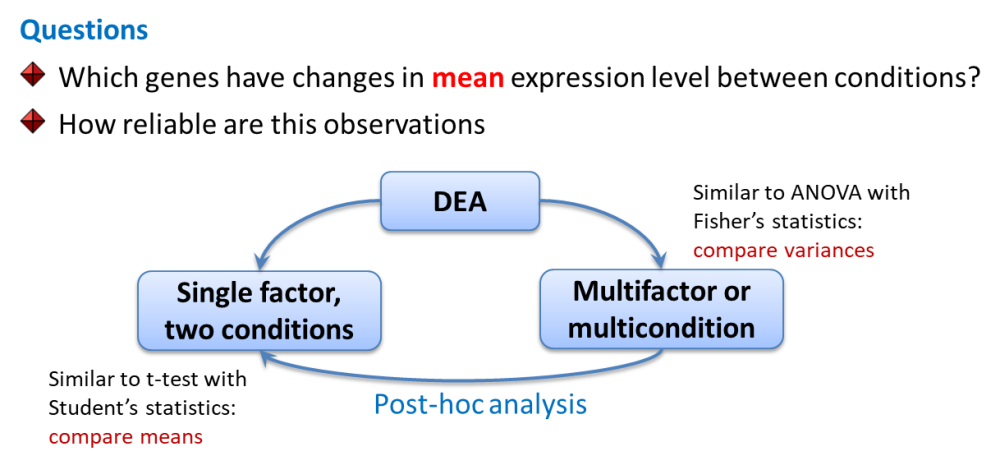
3. Statistics for Transcriptomics

3.1. Installation of the required libraries

Remember:

In the native R, the vast majority of the libraries (or packages) can be simply installed by install.libraries("library_name"). However, some advanced R/Bioconductor packages may need advanced handling of the dependencies. Thus, we would recommend using BiocManager::install() function:

if (!requireNamespace("BiocManager", quietly = TRUE))
    install.packages("BiocManager")

BiocManager::install("limma")
BiocManager::install("edgeR")
BiocManager::install("DESeq2")

DESeq2 (developed in EMBL, Heidelberg) is very powerful but the most demanding package in terms of dependencies :)… Please try to install all 3 packages.

3.2. Analysis of microarrays

General information and data loading

Here we will consider only modern one-color arrays. However the methods were developed and are applicable for two-color arrays.

If you work with Affymetrix (now ThermoFisher) one-colour arrays - be prepared that some preliminary step should be performed before you can really touch the data. Binary CEL files should be processed by one of the tools, probe intensity normalized and summarized into probesets (old arrays and arrays targeted at splicing) or transcript clusters. The later is (to some extent) a synonym for “genes”. Some tools that can help are listed below:

Trancriptome Analysis Console (TAC) - free and quite advanced tool. Allows import Affymetrix and Thermofisher (Clariom) arrays, RMA normalizations with GC correction, data visualization, statistical analysis and functional annotation. (strongly recommended for Affy/Thermo arrays)
Affymetrix Power Tools (APT) - free & flexible command line tools for older versions of Affymetrix arrays.
oligo package of R/Bioconductor - free tool for R geeks :). For example of application - see Exercise 6.1 of AdvBiostat course.

If you would like to check the results of TAC, please see these files:

HTA.txt contains expression measure by HTA 2.0 arrays
HTA_anno.txt - file with annotation.
Sample annotation is in samples.txt

Let’s load mRNA dataset from IFNg experiment

## importing readAMD script from Internet
source("http://r.modas.lu/readAMD.r")

## load mRNA data from IFNg experiment:
mRNA = readAMD("http://edu.modas.lu/data/txt/mrna_ifng.amd.txt",
               stringsAsFactors = TRUE,
               index.column="GeneSymbol",
               sum.func="mean")

`limma` - LInear Models for MicroArrays

Limma works similar to ANOVA with somewhat improved post-hoc analysis and p-value calculation (empirical Bayes statistics). Let’s first see how to do simple analysis and then consider a warp-up function.

DEA approach

library(limma)
library(pheatmap)

## now create design matrix (a lot of "FUN" !)
design = model.matrix(~ -1 + mRNA$meta$time)
colnames(design)=sub(".+time","",colnames(design))
design

##    T00 T03 T12 T24 T48 T72 T72J
## 1    1   0   0   0   0   0    0
## 2    1   0   0   0   0   0    0
## 3    0   1   0   0   0   0    0
## 4    0   1   0   0   0   0    0
## 5    0   0   1   0   0   0    0
## 6    0   0   1   0   0   0    0
## 7    0   0   0   1   0   0    0
## 8    0   0   0   1   0   0    0
## 9    0   0   0   1   0   0    0
## 10   0   0   0   0   1   0    0
## 11   0   0   0   0   1   0    0
## 12   0   0   0   0   1   0    0
## 13   0   0   0   0   0   1    0
## 14   0   0   0   0   0   1    0
## 15   0   0   0   0   0   1    0
## 16   0   0   0   0   0   0    1
## 17   0   0   0   0   0   0    1
## attr(,"assign")
## [1] 1 1 1 1 1 1 1
## attr(,"contrasts")
## attr(,"contrasts")$`mRNA$meta$time`
## [1] "contr.treatment"

## first fit: linear model
fit = lmFit(mRNA$X,design=design)

colnames(design)

## [1] "T00"  "T03"  "T12"  "T24"  "T48"  "T72"  "T72J"

## define contrast (post-hoc of ANOVA)
contrast.matrix = makeContrasts(T03-T00,T12-T00,T24-T00,T48-T00,T72-T00,T72J-T00, levels=design)
contrast.matrix

##       Contrasts
## Levels T03 - T00 T12 - T00 T24 - T00 T48 - T00 T72 - T00 T72J - T00
##   T00         -1        -1        -1        -1        -1         -1
##   T03          1         0         0         0         0          0
##   T12          0         1         0         0         0          0
##   T24          0         0         1         0         0          0
##   T48          0         0         0         1         0          0
##   T72          0         0         0         0         1          0
##   T72J         0         0         0         0         0          1

## second fit: contrasts - like post-hoc in ANOVA
fit2 = contrasts.fit(fit,contrast.matrix)
EB = eBayes(fit2)

## get table of top 100 significant genes by F-statistics (most variable)
Top100 = topTable(EB,coef=NULL,number=100,adjust="BH", genelist = mRNA$anno$GeneSymbol)
str(Top100)

## 'data.frame':    100 obs. of  11 variables:
##  $ ProbeID   : chr  "C1S" "IDO1" "IGFBP5" "C9orf150" ...
##  $ T03...T00 : num  0.78 5.242 -0.112 0.021 1.754 ...
##  $ T12...T00 : num  2.8 7.621 -1.494 0.752 5.454 ...
##  $ T24...T00 : num  4.11 6.84 -2.23 4.25 6.12 ...
##  $ T48...T00 : num  4.7 5.2 -5.99 4.43 4.78 ...
##  $ T72...T00 : num  4.51 3.83 -6.53 4.16 3.64 ...
##  $ T72J...T00: num  0.813 1.1399 -1.7693 0.3305 0.0716 ...
##  $ AveExpr   : num  7.93 8.96 8.68 8.47 8.3 ...
##  $ F         : num  1809 1695 1508 1410 1235 ...
##  $ P.Value   : num  1.98e-21 3.32e-21 8.29e-21 1.41e-20 3.97e-20 ...
##  $ adj.P.Val : num  3.34e-17 3.34e-17 5.57e-17 7.09e-17 1.53e-16 ...

## visualize top 100 by F-stat
genes = Top100[,1]
pheatmap(mRNA$X[genes,],cluster_col=FALSE,fontsize_row=5,fontsize_col=10,cellwidth=15,scale="row",main="Top 100 variable genes (F-stat)")

## get table of top 100 significant genes for the contrast "coef"
Top100 = topTable(EB,coef="T24 - T00",number=100,adjust="BH", genelist = mRNA$anno$GeneSymbol)
str(Top100)

## 'data.frame':    100 obs. of  7 variables:
##  $ ID       : chr  "IDO1" "IRF1" "C1S" "GBP5" ...
##  $ logFC    : num  6.84 5.18 4.11 6.12 4.57 ...
##  $ AveExpr  : num  8.96 10.16 7.93 8.3 11.53 ...
##  $ t        : num  74.5 64.7 62.4 61.8 59.4 ...
##  $ P.Value  : num  1.76e-21 1.59e-20 2.79e-20 3.25e-20 6.07e-20 ...
##  $ adj.P.Val: num  3.54e-17 1.60e-16 1.64e-16 1.64e-16 2.45e-16 ...
##  $ B        : num  37.2 35.7 35.3 35.2 34.7 ...

## visualize top 100 by moderated t-test
genes = Top100[,1]
samples = grep("T00|T24",mRNA$meta$time)
pheatmap(mRNA$X[genes,samples],cluster_col=FALSE,fontsize_row=5,fontsize_col=10,cellwidth=15,scale="row", main="Top 100 genes: T24 - T00 (t-stat)")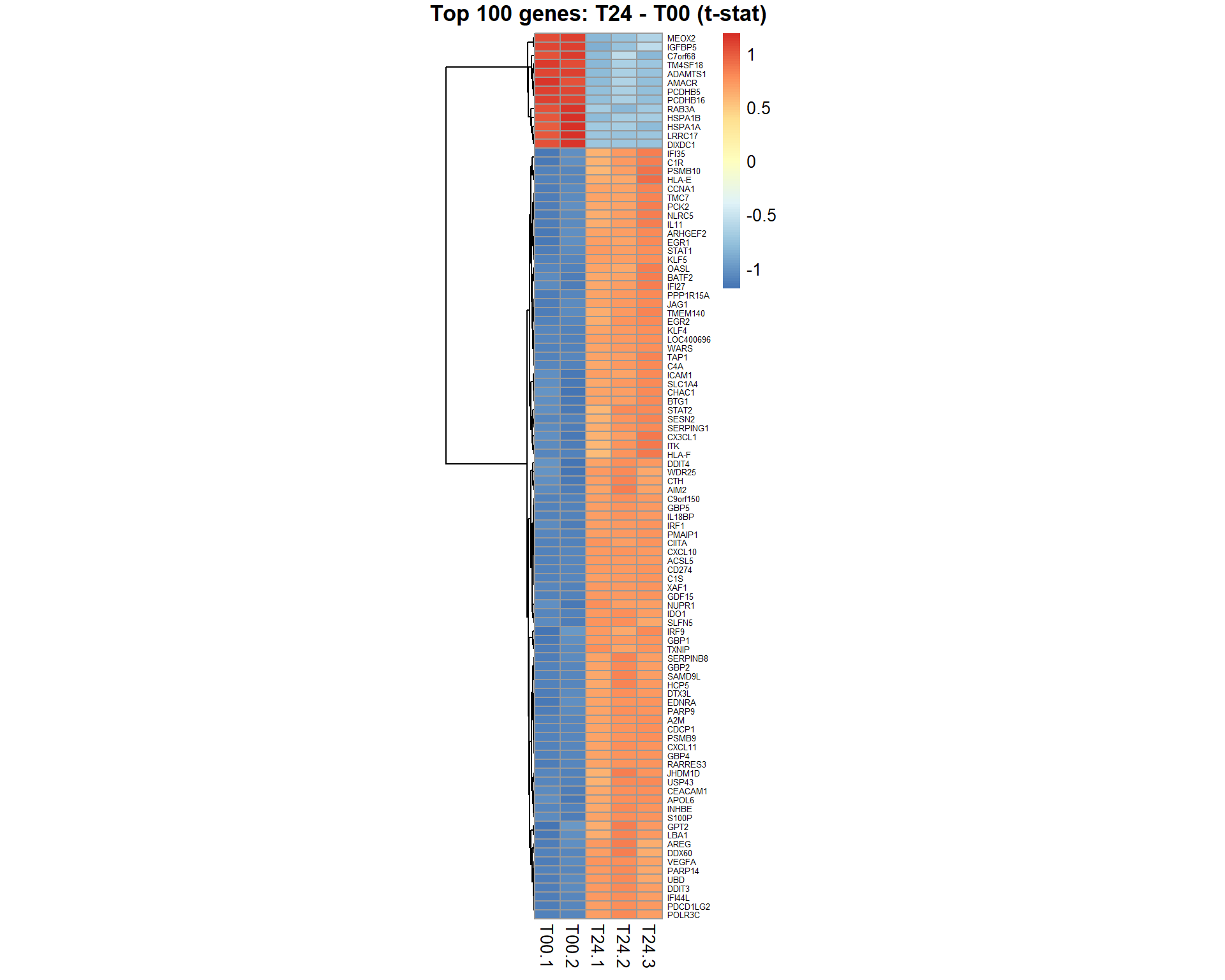

`DEA.limma` - warp-up of the standard limma analysis

Now we do the same with a warp-up function DEA.limma()

source("http://r.modas.lu/LibDEA.r")

## [1] "----------------------------------------------------------------"
## [1] "libDEA: Differential expression analysis"
## [1] "Needed:"
## [1] "limma"    "edgeR"    "DESeq2"   "caTools"  "compiler" "sva"     
## [1] "Absent:"
## character(0)

## most variable (by F-stat)
ResF = DEA.limma(data = mRNA$X, 
                group = mRNA$meta$time)

##  [1] "T03-T00"  "T12-T00"  "T12-T03"  "T24-T00"  "T24-T03"  "T24-T12" 
##  [7] "T48-T00"  "T48-T03"  "T48-T12"  "T48-T24"  "T72-T00"  "T72-T03" 
## [13] "T72-T12"  "T72-T24"  "T72-T48"  "T72J-T00" "T72J-T03" "T72J-T12"
## [19] "T72J-T24" "T72J-T48" "T72J-T72"
## 
## Limma,unpaired: 11468,9604,7444,5630 DEG (FDR<0.05, 1e-2, 1e-3, 1e-4)

str(ResF)

## 'data.frame':    20141 obs. of  26 variables:
##  $ id      : chr  "" "A1BG" "A1CF" "A2BP1" ...
##  $ T03.T00 : num  -0.0237 0.0997 0.0557 -0.033 -0.0733 ...
##  $ T12.T00 : num  0.00463 0.21845 0.11754 -0.06136 -0.27599 ...
##  $ T12.T03 : num  0.0283 0.1188 0.0618 -0.0284 -0.2027 ...
##  $ T24.T00 : num  -0.009247 -0.000912 0.13822 0.055437 0.140712 ...
##  $ T24.T03 : num  0.0144 -0.1006 0.0825 0.0884 0.2141 ...
##  $ T24.T12 : num  -0.0139 -0.2194 0.0207 0.1168 0.4167 ...
##  $ T48.T00 : num  0.0123 0.1058 0.185 0.0644 0.2249 ...
##  $ T48.T03 : num  0.03601 0.00611 0.12927 0.0973 0.29828 ...
##  $ T48.T12 : num  0.00772 -0.11264 0.06747 0.12571 0.50093 ...
##  $ T48.T24 : num  0.02159 0.10672 0.04679 0.00891 0.08422 ...
##  $ T72.T00 : num  -0.0361 0.081 0.0831 0.0756 0.3512 ...
##  $ T72.T03 : num  -0.0125 -0.0187 0.0273 0.1086 0.4245 ...
##  $ T72.T12 : num  -0.0408 -0.1374 -0.0345 0.137 0.6272 ...
##  $ T72.T24 : num  -0.0269 0.0819 -0.0551 0.0202 0.2105 ...
##  $ T72.T48 : num  -0.0485 -0.0248 -0.1019 0.0113 0.1262 ...
##  $ T72J.T00: num  -0.0337 0.0947 0.0557 -0.0732 -0.0356 ...
##  $ T72J.T03: num  -0.01 -0.00504 -0.00004 -0.04028 0.03771 ...
##  $ T72J.T12: num  -0.0383 -0.1238 -0.0618 -0.0119 0.2404 ...
##  $ T72J.T24: num  -0.0244 0.0956 -0.0825 -0.1287 -0.1763 ...
##  $ T72J.T48: num  -0.046 -0.0112 -0.1293 -0.1376 -0.2606 ...
##  $ T72J.T72: num  0.00248 0.01365 -0.02738 -0.14884 -0.38682 ...
##  $ AveExpr : num  6.6 6.25 5.1 4.64 5.92 ...
##  $ F       : num  0.206 1.115 0.752 1.105 12.274 ...
##  $ PValue  : num  9.70e-01 3.97e-01 6.17e-01 4.02e-01 3.62e-05 ...
##  $ FDR     : num  0.974899 0.48257 0.683201 0.487241 0.000126 ...

genes = order(ResF$FDR)[1:100]  ## select top 100 
genes = ResF$id[ResF$FDR < 1e-6] ## select  all significant with FDR<0.000001
pheatmap(mRNA$X[genes,],cluster_col=FALSE,fontsize_row=2,fontsize_col=10,cellwidth=15,scale="row",main="Top 100 variable genes (F-stat)")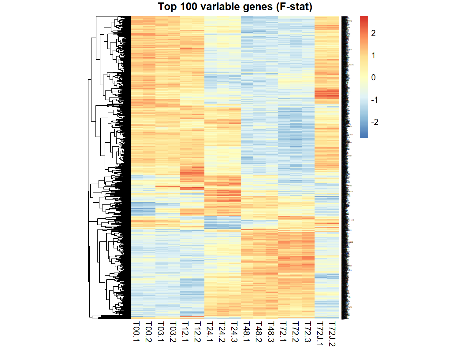

## T24 - T00
Res24 = DEA.limma(data = mRNA$X, 
                group = mRNA$meta$time,
                key0="T00",
                key1="T24")

## 
## Limma,unpaired: 5895,3980,2146,1023 DEG (FDR<0.05, 1e-2, 1e-3, 1e-4)

## now let's plot volcano
plotVolcano(Res24,thr.fdr=0.01,thr.lfc=1)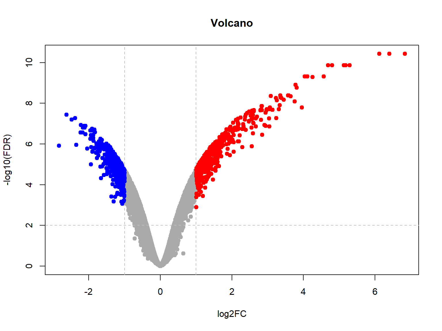

One controversial point is, whether all data should be used for the analysis, or only the one mentioned in the contrast? Often for safety reasons people would like to limit data to the current conditions in the contrast. It decrease sensitivity, but make analysis more robust to changes in other samples.

Finally, let’s save significant data, i.e. with FDR<0.01 to the disk.

str(ResF)
write.table(ResF[ResF$FDR<0.0001,], "DEA_F.txt",col.names=NA,sep="\t",quote=FALSE)

str(Res24)
write.table(Res24[Res24$FDR<0.001 & abs(Res24$logFC)>1,], 
            file = "DEA_T24-T00.txt",col.names=NA,sep="\t",quote=FALSE)

3.3. Functional annotation (to be considered later)

There are tools for functional annotations in R. But for the sake of time, let’s use one of the public tools: Enrichr

Save you significant genes to a file
Put them into the Enrichr tool

write(Res24$id[Res24$FDR<0.001 & abs(Res24$logFC)>1], 
            file = "genes_T24-T00.txt")

3.4. Analysis of RNA-seq data

For simplicity, let’s consider here how to run our custom warp-up function to analyse RNA-Seq data. If you are interested in using original Bioconductor functions - feel free to see in the code of LibDEA

Let’s consider the following libraries:

DESeq2 is the one most often used (subjective), but it is also the slowest one (objective). It needs raw counts (negative binomial model of signal). It is developed by the group of Wolgang Huber (Heidelberg)
edgeR . It needs raw counts (negative binomial model of signal). It is developed by the group of Gordon Smyth (Australia)
limma . It can work with any form of expression (use voom to transform from counts to log-expression). It is as well developed by the group of Gordon Smyth (Australia)

## load data
Data = read.table("http://edu.modas.lu/data/txt/counts.txt",header=T,sep="\t",row.names = 1)
str(Data)

## 'data.frame':    60411 obs. of  18 variables:
##  $ SN327: int  11404 95 5058 4015 4137 266 77088 98 29717 1285 ...
##  $ SN328: int  4652 112 4899 7001 6626 1161 41068 118 13984 1908 ...
##  $ SN349: int  12880 107 5948 6573 4753 523 67236 169 25633 1952 ...
##  $ SN354: int  5252 149 6508 5730 4728 813 56781 250 10469 1830 ...
##  $ SN405: int  7752 169 4596 5858 2926 221 62818 159 13303 1326 ...
##  $ SN449: int  12215 161 4009 4811 3754 620 70614 67 16995 1281 ...
##  $ SN450: int  10898 86 5288 5010 3051 1012 107658 142 20073 1592 ...
##  $ SN667: int  9793 370 4371 4905 3563 118 78049 98 27813 2248 ...
##  $ SN679: int  7039 340 3560 4215 2478 949 62394 120 6482 1036 ...
##  $ ST327: int  1768 32 3346 6450 8849 46 27302 125 165479 1653 ...
##  $ ST328: int  3944 7 5062 6055 5424 1483 24056 185 47563 2947 ...
##  $ ST349: int  4703 54 5837 7117 7773 644 22856 178 94699 2573 ...
##  $ ST354: int  6323 247 8614 5027 8724 83 8912 79 8426 3487 ...
##  $ ST405: int  1496 16 2546 4677 6252 120 27303 143 70070 1364 ...
##  $ ST449: int  5547 33 4912 6942 9630 693 15821 217 87792 2248 ...
##  $ ST450: int  6467 131 5055 4591 7006 1053 33937 101 104311 2242 ...
##  $ ST667: int  2136 43 4608 3955 4599 180 14647 154 41703 1185 ...
##  $ ST679: int  2778 123 1938 1945 2587 909 13117 179 6037 1818 ...

## load annotation
Anno = read.table("http://edu.modas.lu/data/txt/counts_anno.txt",header=T,sep="\t",row.names = 1, as.is=TRUE)
Anno = Anno[rownames(Data),] ## force the same order
str(Anno)

## 'data.frame':    60411 obs. of  8 variables:
##  $ gene_name   : chr  "TSPAN6" "TNMD" "DPM1" "SCYL3" ...
##  $ gene_biotype: chr  "protein_coding" "protein_coding" "protein_coding" "protein_coding" ...
##  $ seqname     : chr  "X" "X" "20" "1" ...
##  $ start       : int  99884983 99839799 49551773 169822913 169631245 27939633 196621008 143816984 53363765 41040684 ...
##  $ stop        : int  99894942 99854882 49574900 169863148 169823221 27961576 196716634 143832548 53481684 41067715 ...
##  $ strand      : chr  "-" "+" "-" "-" ...
##  $ length      : int  2968 1610 1207 3844 6354 3524 8144 2453 8463 3811 ...
##  $ gc          : num  0.441 0.425 0.398 0.445 0.423 ...

This dataset contains 18 samples from 9 lung squamous cell carcinoma patients. Each tumor sample is paired with the normal. Below we will use 3 methods to exptract differentially expessed genes. Feel free to check LibDEA.r for more details.

edgeR - method developed by the same group as limma. It assumes negative binomial distribution of the data
DESeq2 - method developed by W.Huber’s lab in Heidelberg
limma + voom - limma still can be used for counting data

source("http://r.modas.lu/LibDEA.r")

## [1] "----------------------------------------------------------------"
## [1] "libDEA: Differential expression analysis"
## [1] "Needed:"
## [1] "limma"    "edgeR"    "DESeq2"   "caTools"  "compiler" "sva"     
## [1] "Absent:"
## character(0)

group = sub("[0-9]+","",colnames(Data))

## using DESeq2
Res1 = DEA.DESeq(Data, group=group, key0="SN", key1="ST")

## 
## DESeq,unpaired: 11920 DEG (FDR<0.05), 8913 DEG (FDR<0.01)

## using edgeR
Res2 = DEA.edgeR(Data, group=group, key0="SN",key1="ST")

## 
## edgeR,unpaired: 8566 DEG (FDR<0.05), 5990 DEG (FDR<0.01)

## using edgeR
Res3 = DEA.limma(Data, group=group,  key0="SN",key1="ST",counted=TRUE)

## 
## Limma,unpaired: 9038,6004,3329,1767 DEG (FDR<0.05, 1e-2, 1e-3, 1e-4)

The results are not the same. Let’s see:

## Venn diagram
library(gplots)

id1 = Res1[Res1$FDR<0.01 & abs(Res1$logFC)>1,"id"]
id2 = Res2[Res2$FDR<0.01 & abs(Res2$logFC)>1,"id"]
id3 = Res3[Res3$FDR<0.01 & abs(Res3$logFC)>1,"id"]

venn(list(DESeq = id1, edgeR=id2, limma = id3))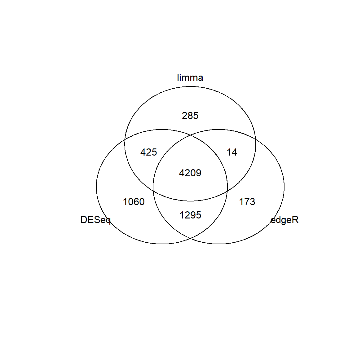

## alternative Venn
# source("http://r.modas.lu/Venn.r")
# v = Venn(list(DESeq = id1, edgeR=id2, limma = id3))

Exercise 3

For mRNA data mRNA, calculate the number of significant genes (FDR<0.01) for each time point vs. T00. Visualize as barplot

DEA.limma(), sum(Res$FDR<0.01), barplot()

Analyze dataset miRNA using either native limma or DEA.limma() warpup. Calculate the number of significant miRNA between untreated samples and each time point.

DEA.limma()

Whether mRNA or miRNA respond faster to IFNg stimulation?

Analyze dataset LUSC60 using one of the methods (DESeq2, edgeR or limma) and compare the gene lists to those found in LIH dataset counts. Sample annotation is quite straitforward: SN - normal, ST - tumour, but can also be found in samples.txt Hint: you will need to translate genes from Ensembl to gene symbols using anno

Alternatively: generate your own “AMD” file in Excel as described in session on Exploratory Data Analysis, section 1.2.1.

DEA.limma,DEA.DESeq,DEA.edgeR sub, venn

Select the top 1000 of the significant genes either in LUSC20 or in counts, save gene names into a file and perform enrichment analysis using Enrichr tool of Icahn School of Medicine at Mount Sinai, NY, USA.

write

Prev Home Next

By Petr Nazarov

3. Statistics for Transcriptomics

Petr V. Nazarov, LIH

2025-02-24

3.1. Installation of the required libraries

3.2. Analysis of microarrays

General information and data loading

`limma` - LInear Models for MicroArrays

`DEA.limma` - warp-up of the standard limma analysis

3.3. Functional annotation (to be considered later)

3.4. Analysis of RNA-seq data

Exercise 3

3. Statistics for Transcriptomics

Petr V. Nazarov, LIH

2025-02-24

3.1. Installation of the required libraries

3.2. Analysis of microarrays

General information and data loading

limma - LInear Models for MicroArrays

DEA.limma - warp-up of the standard limma analysis

3.3. Functional annotation (to be considered later)

3.4. Analysis of RNA-seq data

Exercise 3

`limma` - LInear Models for MicroArrays

`DEA.limma` - warp-up of the standard limma analysis