4. Case study with TAC
Petr V. Nazarov, LIH
2025-02-24
4.1. Functional annotation methods
After we get either the list of significant genes or gene-expression fold change, we would like to understand what these genes mean biologically. Functional annotation allows to make sense from the set of genes. Sets of genes characterize biological processes much better than single genes.
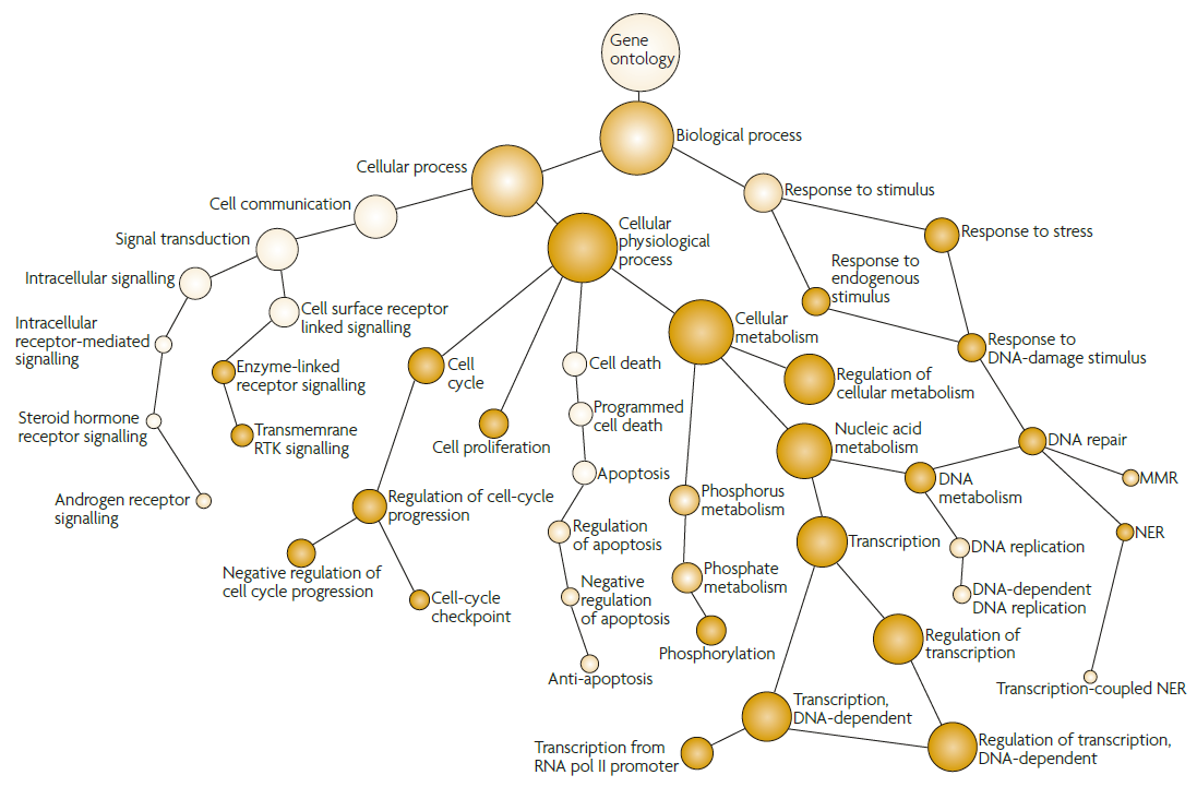
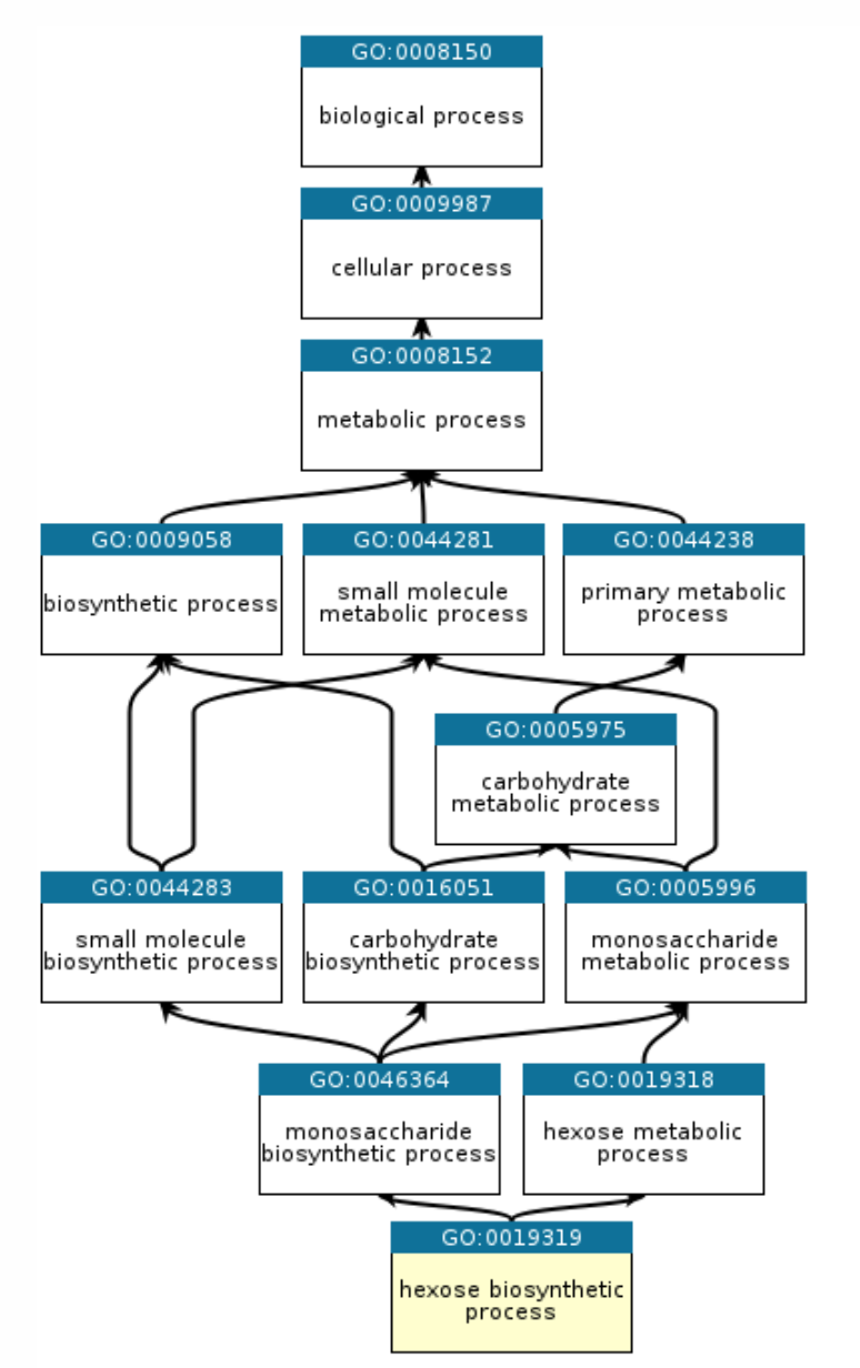
Gene ontology
The Gene Ontology (GO) is a major bioinformatics initiative to unify the representation of gene and gene product attributes across all species. The ontology covers three domains:
Biological Processes - operations or sets of molecular events with a defined beginning and end, pertinent to the functioning of integrated living units
Molecular Functions - the elemental activities of a gene product at the molecular level, such as binding or catalysis
Cellular Components - the parts of a cell or its extracellular environment
Methods
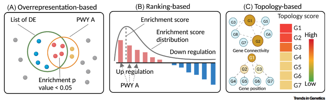
Usually 2 methods are considered [1-2]. Later topology-based method [3] was added
Over-representation Analysis (ORA), e.g. topGO and clusterProfiler
Gene Set Enrichment Analysis (GSEA) e.g. GSEA clusterProfiler
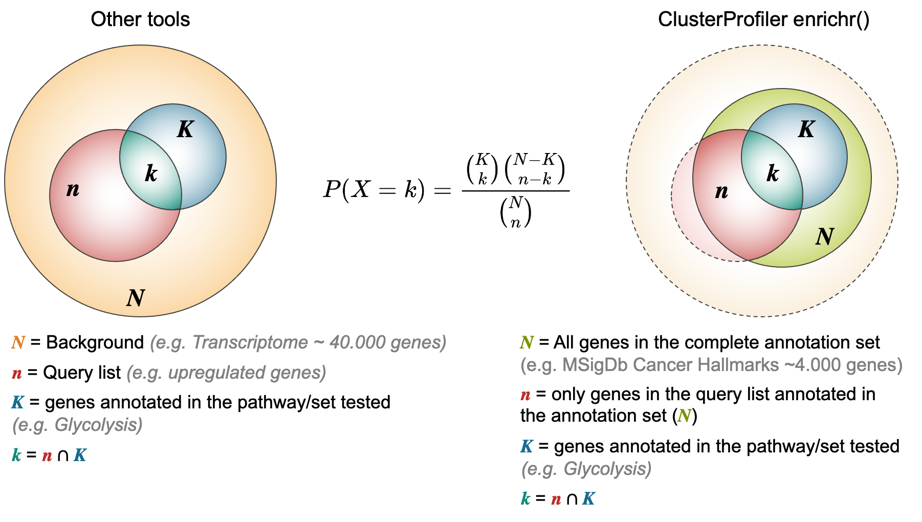
Note regarding ORA:
4.2. Online tools
Enrichr - ORA on many gene sets
David - a comprehensive set of functional annotation tools to help understand the biological meaning behind large gene lists
Reactome - Reactome is a free, open-source, curated and peer-reviewed pathway database
WikiPathways is an open science platform for biological pathways contributed, updated, and used by the research community
4.3. Function annotation in R
Let’s consider how to run functional annotation in R. First - we do
ORA with topGo package. Then - GSEA with
clusterProfiler
ORA in R
source("http://r.modas.lu/LibDEA.r")## [1] "----------------------------------------------------------------"
## [1] "libDEA: Differential expression analysis"
## [1] "Needed:"
## [1] "limma" "edgeR" "DESeq2" "caTools" "compiler" "sva"
## [1] "Absent:"
## character(0)## read the data
Data = read.table("http://edu.modas.lu/data/txt/counts.txt",
header=T,sep="\t",row.names = 1)
str(Data)## 'data.frame': 60411 obs. of 18 variables:
## $ SN327: int 11404 95 5058 4015 4137 266 77088 98 29717 1285 ...
## $ SN328: int 4652 112 4899 7001 6626 1161 41068 118 13984 1908 ...
## $ SN349: int 12880 107 5948 6573 4753 523 67236 169 25633 1952 ...
## $ SN354: int 5252 149 6508 5730 4728 813 56781 250 10469 1830 ...
## $ SN405: int 7752 169 4596 5858 2926 221 62818 159 13303 1326 ...
## $ SN449: int 12215 161 4009 4811 3754 620 70614 67 16995 1281 ...
## $ SN450: int 10898 86 5288 5010 3051 1012 107658 142 20073 1592 ...
## $ SN667: int 9793 370 4371 4905 3563 118 78049 98 27813 2248 ...
## $ SN679: int 7039 340 3560 4215 2478 949 62394 120 6482 1036 ...
## $ ST327: int 1768 32 3346 6450 8849 46 27302 125 165479 1653 ...
## $ ST328: int 3944 7 5062 6055 5424 1483 24056 185 47563 2947 ...
## $ ST349: int 4703 54 5837 7117 7773 644 22856 178 94699 2573 ...
## $ ST354: int 6323 247 8614 5027 8724 83 8912 79 8426 3487 ...
## $ ST405: int 1496 16 2546 4677 6252 120 27303 143 70070 1364 ...
## $ ST449: int 5547 33 4912 6942 9630 693 15821 217 87792 2248 ...
## $ ST450: int 6467 131 5055 4591 7006 1053 33937 101 104311 2242 ...
## $ ST667: int 2136 43 4608 3955 4599 180 14647 154 41703 1185 ...
## $ ST679: int 2778 123 1938 1945 2587 909 13117 179 6037 1818 ...group = sub("[0-9]+","",colnames(Data))
## DEA
Res = DEA.limma(Data, group=group, key0="SN",key1="ST",counted=TRUE)##
## Limma,unpaired: 9038,6004,3329,1767 DEG (FDR<0.05, 1e-2, 1e-3, 1e-4)## Let's find a reasonable number of DEG
table(Res$FDR<0.01)##
## FALSE TRUE
## 54407 6004table(Res$FDR<0.0001, abs(Res$logFC)>1)##
## FALSE TRUE
## FALSE 48046 10598
## TRUE 85 1682## install an use topGO
## install.package("topGO")
## get warp-up with automatic identification fo IDs
source("http://r.modas.lu/enrichGO.r")
## very slow, but hopefully - precise (~ 5 min)
GO = enrichGO(genes =Res$id,
fdr=Res$FDR,
fc=Res$logFC,
ntop=NA,
thr.fdr=0.0001,
thr.fc=1,
db="BP",
genome="org.Hs.eg.db",
do.sort=TRUE)## ntop is NA => using FDR (FC) as limits
## Significant: 1682
## entrez alias ensembl symbol genename
## 0 0 18346 0 0
## Checking DB. The best overlap with [ ensembl ] gene IDs: 18346GO[1:10,]## GO.ID Term Annotated
## GO:0003341 GO:0003341 cilium movement 206
## GO:0035082 GO:0035082 axoneme assembly 96
## GO:0060285 GO:0060285 cilium-dependent cell motility 167
## GO:0044458 GO:0044458 motile cilium assembly 68
## GO:0045841 GO:0045841 negative regulation of mitotic metaphase... 48
## GO:1903047 GO:1903047 mitotic cell cycle process 750
## GO:0006268 GO:0006268 DNA unwinding involved in DNA replicatio... 21
## GO:0044782 GO:0044782 cilium organization 410
## GO:0034508 GO:0034508 centromere complex assembly 28
## GO:0001953 GO:0001953 negative regulation of cell-matrix adhes... 36
## Significant Expected classicFisher FDR Score
## GO:0003341 79 11.32 1.0e-31 7.740500e-28 27.111231
## GO:0035082 55 5.27 1.0e-31 7.740500e-28 27.111231
## GO:0060285 58 9.18 1.7e-30 8.772567e-27 26.056873
## GO:0044458 28 3.74 4.4e-18 1.702910e-14 13.768808
## GO:0045841 17 2.64 2.8e-10 8.669360e-07 6.062013
## GO:1903047 118 41.21 3.0e-09 7.740500e-06 5.111231
## GO:0006268 10 1.15 4.9e-08 1.083670e-04 3.965103
## GO:0044782 100 22.53 9.9e-08 1.915774e-04 3.717656
## GO:0034508 11 1.54 1.2e-07 2.064133e-04 3.685262
## GO:0001953 12 1.98 2.6e-07 4.025060e-04 3.395228GSEA in R
We will use a powerful packageclusterProfiler
library(clusterProfiler)
library(enrichplot)
library(ggplot2)
organism = "org.Hs.eg.db"
library(organism, character.only = TRUE)
library(msigdbr)

## let's use previously calculated Res
str(Res)
## 'data.frame': 60411 obs. of 7 variables:
## $ id : chr "ENSG00000000003" "ENSG00000000005" "ENSG00000000419" "ENSG00000000457" ...
## $ logFC : num -1.0714 -1.4679 0.0624 0.1187 0.944 ...
## $ AveExpr: num 5.343 -0.638 5.088 5.245 5.204 ...
## $ t : num -4.6 -2.722 0.454 0.721 4.932 ...
## $ PValue : num 2.00e-04 1.36e-02 6.55e-01 4.80e-01 9.52e-05 ...
## $ FDR : num 0.00279 0.07887 0.73347 0.57084 0.00153 ...
## $ B : num 0.136 -3.311 -7.144 -7.001 0.895 ...logfc = Res$logFC
names(logfc) = Res$id ## here we have genes given as Ensembl ID
## deal with zeros - exlude
logfc = logfc[logfc!=0]
## sort the list in decreasing order (required for clusterProfiler)
logfc = sort(logfc, decreasing = TRUE)
## see all MSIGdb names
as.data.frame(msigdbr_collections())## gs_cat gs_subcat num_genesets
## 1 C1 299
## 2 C2 CGP 3384
## 3 C2 CP 29
## 4 C2 CP:BIOCARTA 292
## 5 C2 CP:KEGG 186
## 6 C2 CP:PID 196
## 7 C2 CP:REACTOME 1615
## 8 C2 CP:WIKIPATHWAYS 664
## 9 C3 MIR:MIRDB 2377
## 10 C3 MIR:MIR_Legacy 221
## 11 C3 TFT:GTRD 518
## 12 C3 TFT:TFT_Legacy 610
## 13 C4 CGN 427
## 14 C4 CM 431
## 15 C5 GO:BP 7658
## 16 C5 GO:CC 1006
## 17 C5 GO:MF 1738
## 18 C5 HPO 5071
## 19 C6 189
## 20 C7 IMMUNESIGDB 4872
## 21 C7 VAX 347
## 22 C8 700
## 23 H 50## storage
GSEA = list()
icol=1
for (icol in 1:nrow(msigdbr_collections())){
name = paste(as.vector(as.matrix(msigdbr_collections()[icol,1:2])),collapse="|")
print(name)
gs_cat = data.frame(msigdbr_collections())[icol,1]
gs_subcat = data.frame(msigdbr_collections())[icol,2]
gsdf = data.frame(msigdbr(species = "Homo sapiens",category=gs_cat,subcategory=gs_subcat))
gsdf = gsdf[gsdf$human_ensembl_gene %in% names(logfc),
c("gs_name","gs_description","gene_symbol","human_ensembl_gene")]
gsea = GSEA(geneList=logfc[names(logfc) %in% gsdf[,4]],
eps=1e-20,
TERM2GENE = gsdf[,c(1,4)],
TERM2NAME = gsdf[,c(1,2)],
pvalueCutoff = 0.1)
GSEA[[name]] = gsea@result
rownames(GSEA[[name]]) = GSEA[[name]]$ID
}## [1] "C1|"## [1] "C2|CGP"## [1] "C2|CP"## [1] "C2|CP:BIOCARTA"## [1] "C2|CP:KEGG"## [1] "C2|CP:PID"## [1] "C2|CP:REACTOME"## [1] "C2|CP:WIKIPATHWAYS"## [1] "C3|MIR:MIRDB"## [1] "C3|MIR:MIR_Legacy"## [1] "C3|TFT:GTRD"## [1] "C3|TFT:TFT_Legacy"## [1] "C4|CGN"## [1] "C4|CM"## [1] "C5|GO:BP"## [1] "C5|GO:CC"## [1] "C5|GO:MF"## [1] "C5|HPO"## [1] "C6|"## [1] "C7|IMMUNESIGDB"## [1] "C7|VAX"## [1] "C8|"## [1] "H|" ## save your results
saveRDS(GSEA,file=sprintf("GSEA.rds"))Now you can investigate your GSEA object.
| Prev Home Prev |
By Petr Nazarov
|