Video 1-2

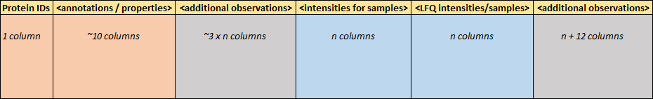
1.1. Main data formats

In bioinformatics people prefer using plain text format for the data (obvious reason…). Main formats are TSV and CSV.

Some binary formats you may easily use as well.

Example TSV:

## let's read this file from internet
Mice = read.table("http://edu.modas.lu/data/txt/mice.txt",
                  sep = "\t",
                  header= TRUE,
                  stringsAsFactors = TRUE)
str(Mice)
## 'data.frame':    790 obs. of  14 variables:
##  $ ID                  : int  1 2 3 368 369 370 371 372 4 5 ...
##  $ Strain              : Factor w/ 40 levels "129S1/SvImJ",..: 1 1 1 1 1 1 1 1 1 1 ...
##  $ Sex                 : Factor w/ 2 levels "f","m": 1 1 1 1 1 1 1 1 1 1 ...
##  $ Starting.age        : int  66 66 66 72 72 72 72 72 66 66 ...
##  $ Ending.age          : int  116 116 108 114 115 116 119 122 109 112 ...
##  $ Starting.weight     : num  19.3 19.1 17.9 18.3 20.2 18.8 19.4 18.3 17.2 19.7 ...
##  $ Ending.weight       : num  20.5 20.8 19.8 21 21.9 22.1 21.3 20.1 18.9 21.3 ...
##  $ Weight.change       : num  1.06 1.09 1.11 1.15 1.08 ...
##  $ Bleeding.time       : int  64 78 90 65 55 NA 49 73 41 129 ...
##  $ Ionized.Ca.in.blood : num  1.2 1.15 1.16 1.26 1.23 1.21 1.24 1.17 1.25 1.14 ...
##  $ Blood.pH            : num  7.24 7.27 7.26 7.22 7.3 7.28 7.24 7.19 7.29 7.22 ...
##  $ Bone.mineral.density: num  0.0605 0.0553 0.0546 0.0599 0.0623 0.0626 0.0632 0.0592 0.0513 0.0501 ...
##  $ Lean.tissues.weight : num  14.5 13.9 13.8 15.4 15.6 16.4 16.6 16 14 16.3 ...
##  $ Fat.weight          : num  4.4 4.4 2.9 4.2 4.3 4.3 5.4 4.1 3.2 5.2 ...

Example CSV:

BC = read.csv("http://edu.modas.lu/data/txt/breastcancer.csv",
              comment.char="#",  
              header= TRUE)
str(BC)
## 'data.frame':    699 obs. of  11 variables:
##  $ sample         : int  1000025 1002945 1015425 1016277 1017023 1017122 1018099 1018561 1033078 1033078 ...
##  $ clump.thickness: int  5 5 3 6 4 8 1 2 2 4 ...
##  $ uni.size       : int  1 4 1 8 1 10 1 1 1 2 ...
##  $ uni.shape      : int  1 4 1 8 1 10 1 2 1 1 ...
##  $ adhesion       : int  1 5 1 1 3 8 1 1 1 1 ...
##  $ epith.size     : int  2 7 2 3 2 7 2 2 2 2 ...
##  $ bare.nuclei    : int  1 10 2 4 1 10 10 1 1 1 ...
##  $ bland.chromatin: int  3 3 3 3 3 9 3 3 1 2 ...
##  $ normal.nucleoli: int  1 2 1 7 1 7 1 1 1 1 ...
##  $ mitoses        : int  1 1 1 1 1 1 1 1 5 1 ...
##  $ class          : int  0 0 0 0 0 1 0 0 0 0 ...

Example Excel:

# install.packages("readxl")
library(readxl)

## download Excel file and store it locally
download.file("http://edu.modas.lu/data/xls/cancer.xlsx",destfile="cancer.xlsx",mode = "wb")

## read Excel file into `tibble`
Cancer = read_excel("cancer.xlsx") 
str(Cancer)

## optional: change to `data.frame`
Cancer = as.data.frame(Cancer)

1.2. Custom formats

1.2.1. Merged: Annotation-Metadata-Data

This is a custom format I used together with some collaborators to simplify sample annotation

Example:

## load the function from Internet
source("http://r.modas.lu/readAMD.r")  

## read AMD-file from Internet:
miR = readAMD("http://edu.modas.lu/data/txt/mirna_ifng.amd.txt",stringsAsFactors=TRUE)
str(miR)
## List of 5
##  $ ncol: int 20
##  $ nrow: int 2226
##  $ anno:'data.frame':    2226 obs. of  7 variables:
##   ..$ ID                         : chr [1:2226] "hp_hsa-let-7a-1_st" "hp_hsa-let-7a-1_x_st" "hp_hsa-let-7a-2_st" "hp_hsa-let-7a-2_x_st" ...
##   ..$ Alignments                 : chr [1:2226] "9:96938239-96938318 (+)" "9:96938239-96938318 (+)" "11:122017230-122017301 (-)" "11:122017230-122017301 (-)" ...
##   ..$ Sequence                   : chr [1:2226] "TGGGATGAGGTAGTAGGTTGTATAGTTTTAGGGTCACACCCACCACTGGGAGATAACTATACAATCTACTGTCTTTCCTA" "TGGGATGAGGTAGTAGGTTGTATAGTTTTAGGGTCACACCCACCACTGGGAGATAACTATACAATCTACTGTCTTTCCTA" "AGGTTGAGGTAGTAGGTTGTATAGTTTAGAATTACATCAAGGGAGATAACTGTACAGCCTCCTAGCTTTCCT" "AGGTTGAGGTAGTAGGTTGTATAGTTTAGAATTACATCAAGGGAGATAACTGTACAGCCTCCTAGCTTTCCT" ...
##   ..$ Sequence.Length            : int [1:2226] 80 80 72 72 74 83 83 84 84 87 ...
##   ..$ Sequence.Type              : chr [1:2226] "stem-loop" "stem-loop" "stem-loop" "stem-loop" ...
##   ..$ Species.Scientific.Name    : chr [1:2226] "Homo sapiens" "Homo sapiens" "Homo sapiens" "Homo sapiens" ...
##   ..$ Transcript.ID.Array.Design.: chr [1:2226] "hsa-let-7a-1" "hsa-let-7a-1" "hsa-let-7a-2" "hsa-let-7a-2" ...
##  $ meta:'data.frame':    20 obs. of  2 variables:
##   ..$ time     : Factor w/ 10 levels "T00","T005","T03",..: 1 1 2 2 3 3 4 4 5 5 ...
##   ..$ replicate: Factor w/ 2 levels "r1","r2": 1 2 1 2 1 2 1 2 1 2 ...
##  $ X   : num [1:2226, 1:20] 2.75 1.318 1.995 1.696 0.906 ...
##   ..- attr(*, "dimnames")=List of 2
##   .. ..$ : chr [1:2226] "hp_hsa-let-7a-1_st" "hp_hsa-let-7a-1_x_st" "hp_hsa-let-7a-2_st" "hp_hsa-let-7a-2_x_st" ...
##   .. ..$ : chr [1:20] "T000.1" "T000.2" "T005.1" "T005.2" ...
## reading & parsing large text files Internet can be long.
## => often it is better to download and read text-file from local storage.
## However, readAMD() includes downloading

mRNA = readAMD("http://edu.modas.lu/data/txt/mrna_ifng.amd.txt",stringsAsFactors=TRUE) 
str(mRNA)
## List of 5
##  $ ncol: int 17
##  $ nrow: int 33297
##  $ anno:'data.frame':    33297 obs. of  8 variables:
##   ..$ ID             : int [1:33297] 7892501 7892502 7892503 7892504 7892505 7892506 7892507 7892508 7892509 7892510 ...
##   ..$ gene_assignment: chr [1:33297] "---" "---" "---" "---" ...
##   ..$ GeneSymbol     : chr [1:33297] "" "" "" "" ...
##   ..$ RefSeq         : chr [1:33297] "---" "---" "---" "---" ...
##   ..$ seqname        : chr [1:33297] "---" "---" "---" "---" ...
##   ..$ start          : int [1:33297] 0 0 0 0 0 0 0 0 0 0 ...
##   ..$ stop           : int [1:33297] 0 0 0 0 0 0 0 0 0 0 ...
##   ..$ strand         : chr [1:33297] "---" "---" "---" "---" ...
##  $ meta:'data.frame':    17 obs. of  3 variables:
##   ..$ time     : Factor w/ 7 levels "T00","T03","T12",..: 1 1 2 2 3 3 4 4 4 5 ...
##   ..$ treatment: Factor w/ 3 levels "IFNg","IFNg_JII",..: 3 3 1 1 1 1 1 1 1 1 ...
##   ..$ replicate: Factor w/ 3 levels "r1","r2","r3": 1 2 1 2 1 2 1 2 3 1 ...
##  $ X   : num [1:33297, 1:17] 9.21 7.64 5 8.57 7.1 ...
##   ..- attr(*, "dimnames")=List of 2
##   .. ..$ : chr [1:33297] "7892501" "7892502" "7892503" "7892504" ...
##   .. ..$ : chr [1:17] "T00.1" "T00.2" "T03.1" "T03.2" ...

It looks like many probesets (rows) are not annotated… Let’s summarize the data to GeneSymbol.

mRNA = readAMD("d:/data/r/mrna_ifng.amd.txt", ## put you path to the file
              stringsAsFactors=TRUE,
              index.column="GeneSymbol",
              sum.func="mean")
  str(mRNA)
## List of 5
##  $ ncol: int 17
##  $ nrow: int 20141
##  $ anno:'data.frame':    20141 obs. of  8 variables:
##   ..$ GeneSymbol     : chr [1:20141] "" "A1BG" "A1CF" "A2BP1" ...
##   ..$ ID             : chr [1:20141] "7892501,7892502,7892503,7892504,7892505,7892506,7892507,7892508,7892509,7892510,7892511,7892512,7892513,7892514"| __truncated__ "8039748" "7933640" "7993083,7993110" ...
##   ..$ gene_assignment: chr [1:20141] "---," "NM_130786 // A1BG // alpha-1-B glycoprotein // 19q13.4 // 1 /// NM_198458 // ZNF497 // zinc finger protein 497 "| __truncated__ "NM_138933 // A1CF // APOBEC1 complementation factor // 10q11.23 // 29974 /// NM_014576 // A1CF // APOBEC1 compl"| __truncated__ "NM_018723 // A2BP1 // ataxin 2-binding protein 1 // 16p13.3 // 54715 /// NM_145893 // A2BP1 // ataxin 2-binding"| __truncated__ ...
##   ..$ RefSeq         : chr [1:20141] "---," "NM_130786" "NM_138933" "NM_018723,ENST00000432184" ...
##   ..$ seqname        : chr [1:20141] "---,chr1,chr10,,chr11,chr12,chr13,chrUn_gl000212,chr14,chr15,chr16,chr17,chr17_gl000205_random,chr18,chr19,chr2"| __truncated__ "chr19" "chr10" "chr16" ...
##   ..$ start          : chr [1:20141] "        0,    53049,    63015,   564951,   566062,   568844,  1102484,  1103243,  1104373,  2316811,  6600914, "| __truncated__ " 58856544" " 52566314" "  6069132,  6753884" ...
##   ..$ stop           : chr [1:20141] "        0,    54936,    63887,   565019,   566129,   568913,  1102578,  1103332,  1104471,  2319922,  6600994, "| __truncated__ " 58867591" " 52645435" "  7763340,  6755559" ...
##   ..$ strand         : chr [1:20141] "---,+,-," "-" "-" "+" ...
##  $ meta:'data.frame':    17 obs. of  2 variables:
##   ..$ time     : Factor w/ 7 levels "T00","T03","T12",..: 1 1 2 2 3 3 4 4 4 5 ...
##   ..$ replicate: Factor w/ 3 levels "r1","r2","r3": 1 2 1 2 1 2 1 2 3 1 ...
##  $ X   : num [1:20141, 1:17] 6.6 6.15 5.1 4.64 5.78 ...
##   ..- attr(*, "dimnames")=List of 2
##   .. ..$ : chr [1:20141] "" "A1BG" "A1CF" "A2BP1" ...
##   .. ..$ : chr [1:17] "T00.1" "T00.2" "T03.1" "T03.2" ...

1.2.2. Read MaxQuant results (proteomics)

Another example - MaxQuant file, which is the result of spectra analysis in MS/MS spectrometry. It contains inferred protein groups in the samples with a lot of other annotation.

MaxQuant protein-group file

You can read such data using read.table() and then process, or write (ask to write) a small function for data import:

source("http://r.modas.lu/readMaxQuant.r")  ## function

Prot = readMaxQuant("http://edu.modas.lu/data/txt/proteingroups.txt")
## 1484 features were read.
## Reverse and contaminants are removed, resulting in 1433 features 
## Remove 4 uninformative features
## ` LFQ.intensity. ` was extracted for 12 samples.
str(Prot)
## List of 6
##  $ nf  : int 1429
##  $ ns  : int 12
##  $ Anno:'data.frame':    1429 obs. of  5 variables:
##   ..$ Majority.protein.IDs: chr [1:1429] "H0Y9X3;A0A024QZ42;A0A087WZ38;O75340" "P06493;A0A024QZP7;A0A087WZZ9" "A0A024R4E5;Q00341;H0Y394;H7C2D1" "A0A024R4M0;P46781;B5MCT8;C9JM19" ...
##   ..$ Protein.names       : chr [1:1429] "Programmed cell death protein 6" "Cyclin-dependent kinase 1" "Vigilin" "40S ribosomal protein S9" ...
##   ..$ Gene.names          : chr [1:1429] "PDCD6" "CDK1;CDC2" "HDLBP" "RPS9" ...
##   ..$ Fasta.headers       : chr [1:1429] "tr|H0Y9X3|H0Y9X3_HUMAN Programmed cell death protein 6 (Fragment) OS=Homo sapiens OX=9606 GN=PDCD6 PE=1 SV=1;tr"| __truncated__ "sp|P06493|CDK1_HUMAN Cyclin-dependent kinase 1 OS=Homo sapiens OX=9606 GN=CDK1 PE=1 SV=3;tr|A0A024QZP7|A0A024QZ"| __truncated__ "tr|A0A024R4E5|A0A024R4E5_HUMAN High density lipoprotein binding protein (Vigilin), isoform CRA_a OS=Homo sapien"| __truncated__ "tr|A0A024R4M0|A0A024R4M0_HUMAN 40S ribosomal protein S9 OS=Homo sapiens OX=9606 GN=RPS9 PE=1 SV=1;sp|P46781|RS9"| __truncated__ ...
##   ..$ Number.of.proteins  : int [1:1429] 4 29 12 6 5 2 2 9 9 2 ...
##  $ Meta:'data.frame':    12 obs. of  1 variable:
##   ..$ ID: chr [1:12] "136.R1" "136.R2" "136.R3" "136.R4" ...
##  $ X0  : num [1:1429, 1:12] 0.00 0.00 0.00 1.08e+08 2.20e+06 ...
##   ..- attr(*, "dimnames")=List of 2
##   .. ..$ : chr [1:1429] "H0Y9X3;A0A024QZ42;A0A087WZ38;O75340" "P06493;A0A024QZP7;A0A087WZZ9;E5RIU6;E7ESI2;F5H6Z0;A0A087WZU2;E5RGN0;G3V5T9;E7EUK8;K7ELV5;H0YAZ9;K7EJ83;F8VYH9;F"| __truncated__ "A0A024R4E5;Q00341;H0Y394;H7C2D1;C9JT62;C9JHS7;C9JK79;C9JHZ8;C9JES8;C9JZI8;C9J5E5;C9JIZ1" "A0A024R4M0;P46781;B5MCT8;C9JM19;F2Z3C0;A8MXK4" ...
##   .. ..$ : chr [1:12] "136.R1" "136.R2" "136.R3" "136.R4" ...
##  $ LX  : num [1:1429, 1:12] 0 0 0 7.68 2.36 ...
##   ..- attr(*, "dimnames")=List of 2
##   .. ..$ : chr [1:1429] "H0Y9X3;A0A024QZ42;A0A087WZ38;O75340" "P06493;A0A024QZP7;A0A087WZZ9;E5RIU6;E7ESI2;F5H6Z0;A0A087WZU2;E5RGN0;G3V5T9;E7EUK8;K7ELV5;H0YAZ9;K7EJ83;F8VYH9;F"| __truncated__ "A0A024R4E5;Q00341;H0Y394;H7C2D1;C9JT62;C9JHS7;C9JK79;C9JHZ8;C9JES8;C9JZI8;C9J5E5;C9JIZ1" "A0A024R4M0;P46781;B5MCT8;C9JM19;F2Z3C0;A8MXK4" ...
##   .. ..$ : chr [1:12] "136.R1" "136.R2" "136.R3" "136.R4" ...

1.2.3. Read configuration (*.ini) files

Some times you may need read and write some configuration of the analysis. One of the options - use .ini or .cfg files. Here is an example how to read configuration from an INI file:

source("http://r.modas.lu/parseINI.r")  

INI = parseINI("http://edu.modas.lu/data/simple.ini")

print(INI)
## $`Section 1`
## $`Section 1`$key1
## [1] "Hello"
## 
## $`Section 1`$key2
## [1] "2020"
## 
## 
## $`Section 2`
## $`Section 2`$key3
## [1] "0.05"
## 
## $`Section 2`$key4
## [1] "TRUE"
## 
## $`Section 2`$key5
## [1] "A,B,C,D"

1.3. Images

# install.packages("jpeg")
library(jpeg)

## define rotation to orient image properly
rotate <- function(x) t(apply(x, 2, rev))

## download image
download.file("http://edu.modas.lu/data/img/stainhe_gtexpanreas.jpg",
              destfile = "stainhe_gtexpanreas.jpg",
              mode = "wb")

## read image in 3D array (matrix)
A = readJPEG("stainhe_gtexpanreas.jpg")

str(A)
##  num [1:771, 1:1254, 1:3] 0.761 0.753 0.525 0.31 0.267 ...
## show image and 3 channels
par(mfcol=c(2,2))
plot.new()
rasterImage(A, 0, 0, 1, 1)
image(rotate(A[,,1]),main="Red",col=gray.colors(256))
image(rotate(A[,,2]),main="Green",col=gray.colors(256))
image(rotate(A[,,3]),main="Blue",col=gray.colors(256))

## zoom in
par(mfcol=c(2,2))
plot.new()
rasterImage(A[500:700,500:700,], 0, 0, 1, 1)
image(rotate(A[500:700,500:700,1]),main="Red",col=gray.colors(256))
image(rotate(A[500:700,500:700,2]),main="Green",col=gray.colors(256))
image(rotate(A[500:700,500:700,3]),main="Blue",col=gray.colors(256))


Home Next

By Petr Nazarov