3. Dimensionality reduction

You should have loaded the following data:

Mice - mouse phenome dataset (790 mice)
miR & mRNA - microRNA and mRNA profiles of A375 cell line after stimulation with IFNg (adapted from [Nazarov et al, Nucleic Acid Research, 2013])

If not, please load:

## load the script from Internet
source("http://r.modas.lu/readAMD.r")

## Mouse 'phenome' data
Mice = read.table("http://edu.modas.lu/data/txt/mice.txt",
                  sep="\t",
                  header=TRUE,
                  stringsAsFactors = TRUE)

## miRNA data
miR = readAMD("http://edu.modas.lu/data/txt/mirna_ifng.amd.txt",stringsAsFactors = TRUE)

## mRNA data
mRNA = readAMD("http://edu.modas.lu/data/txt/mrna_ifng.amd.txt",
               stringsAsFactors = TRUE,
               index.column="GeneSymbol",
               sum.func="mean")

3.1. Overview of dimensionality reduction methods

Some of the most used dimensionality reduction methods

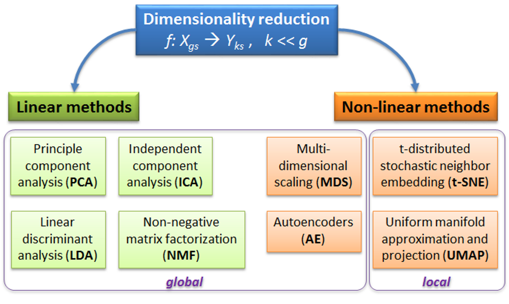
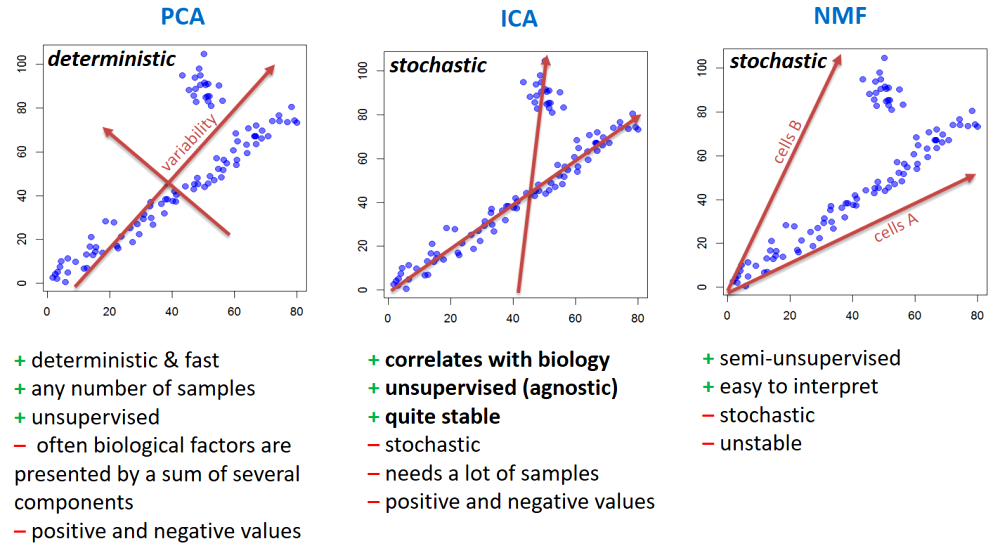
PCA - rotation of the coordinate system in multidimensional space in the way to capture main variability in the data.
ICA - matrix factorization method that identifies statistically independent signals and their weights.
NMF - matrix factorization method that presents data as a matrix product of two non-negative matrices.
LDA - identify new coordinate system, maximizing difference between objects belonging to predefined groups.
MDS - method that tries to preserve distances between objects in the low-dimension space.
AE - artificial neural network with a “bottle-neck”.
t-SNE - an iterative approach, similar to MDS, but consideting only close objects. Thus, similar objects must be close in the new (reduced) space, while distant objects are not influecing the results.
UMAP - modern method, similar to t-SNE, but more stable and with preservation of some information about distant groups (preserving topology of the data).

Comparing PCA, ICA and NMF. See also Sompairac et al, Mol.Sci., 2019

Let’s consider some nice resources online:

Principal Component Analysis Explained Visually by Victor Powell
Understanding UMAP by Andy Coenen and Adam Pearce
Dimensionality Reduction for Data Visualization: PCA vs TSNE vs UMAP vs LDA by Sivakar Sivarajah

3.2. PCA - Principle Component Analysis

3.2.1 PCA of samples in the space of features (genes/proteins)

Simplest way to do PCA in R is to use default prcomp() function. It takes a matrix with samples in rows and features in columns.

If you assume that absolute values of features is not important (only relative variability) - use scale=TRUE.

PC = prcomp(t(mRNA$X),scale=TRUE) 
str(PC)

## List of 5
##  $ sdev    : num [1:17] 83.4 55.3 48.1 42 36 ...
##  $ rotation: num [1:20141, 1:17] 0.001125 0.000754 0.006407 0.008881 0.009878 ...
##   ..- attr(*, "dimnames")=List of 2
##   .. ..$ : chr [1:20141] "" "A1BG" "A1CF" "A2BP1" ...
##   .. ..$ : chr [1:17] "PC1" "PC2" "PC3" "PC4" ...
##  $ center  : Named num [1:20141] 6.6 6.25 5.1 4.64 5.92 ...
##   ..- attr(*, "names")= chr [1:20141] "" "A1BG" "A1CF" "A2BP1" ...
##  $ scale   : Named num [1:20141] 0.0233 0.1059 0.1061 0.0862 0.2095 ...
##   ..- attr(*, "names")= chr [1:20141] "" "A1BG" "A1CF" "A2BP1" ...
##  $ x       : num [1:17, 1:17] -84.9 -104.8 -69.3 -81.6 -70 ...
##   ..- attr(*, "dimnames")=List of 2
##   .. ..$ : chr [1:17] "T00.1" "T00.2" "T03.1" "T03.2" ...
##   .. ..$ : chr [1:17] "PC1" "PC2" "PC3" "PC4" ...
##  - attr(*, "class")= chr "prcomp"

plot(PC$x[,"PC1"],PC$x[,"PC2"],col=as.integer(mRNA$meta$time),pch=19,cex=2,
     main="PCA (scaled gene expression)")

Alternatively you could use my warp-up function plotPCA(). Let’s try it with and without gene scaling

source("http://sablab.net/scripts/plotPCA.r")
par(mfcol=c(1,2))
plotPCA(mRNA$X,col=as.integer(mRNA$meta$time),cex.names=1,cex=2, 
        main="PCA (gene scaling)")
plotPCA(mRNA$X,col=as.integer(mRNA$meta$time),cex.names=1,cex=2, scale=FALSE,
        main="PCA (no scaling)")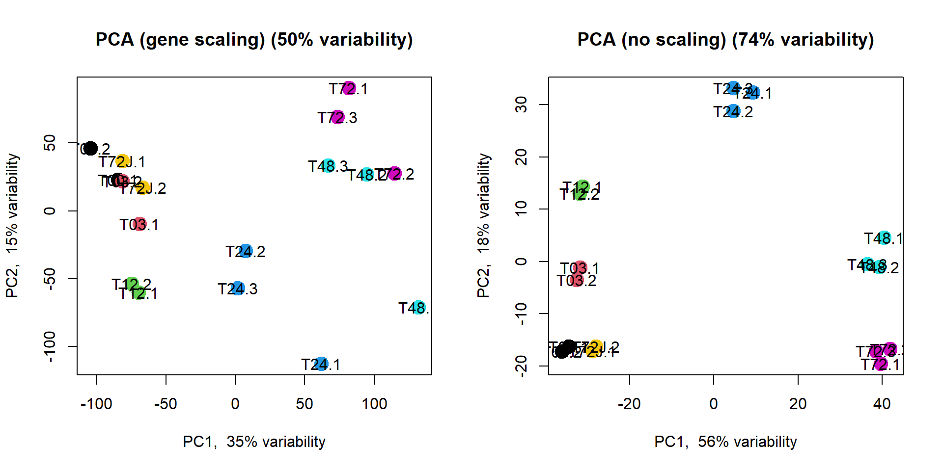

Variability captured by each component can be calculated and visualized as a scree plot manualy:

## calculate percentage of variability
PC$pvar = (PC$sdev^2)/sum(PC$sdev^2)
names(PC$pvar) = colnames(PC$x)

## draw scree plot
barplot(PC$pvar[1:10],ylim = c(0,0.4), col="skyblue",main="Explained Variability",cex.main=1, xlab="Components",ylab="Variability explained")

## add text
text(1.2 * (1:10)-0.5,PC$pvar[1:10],sprintf("%.3f",PC$pvar[1:10]),adj=c(0.5,-1))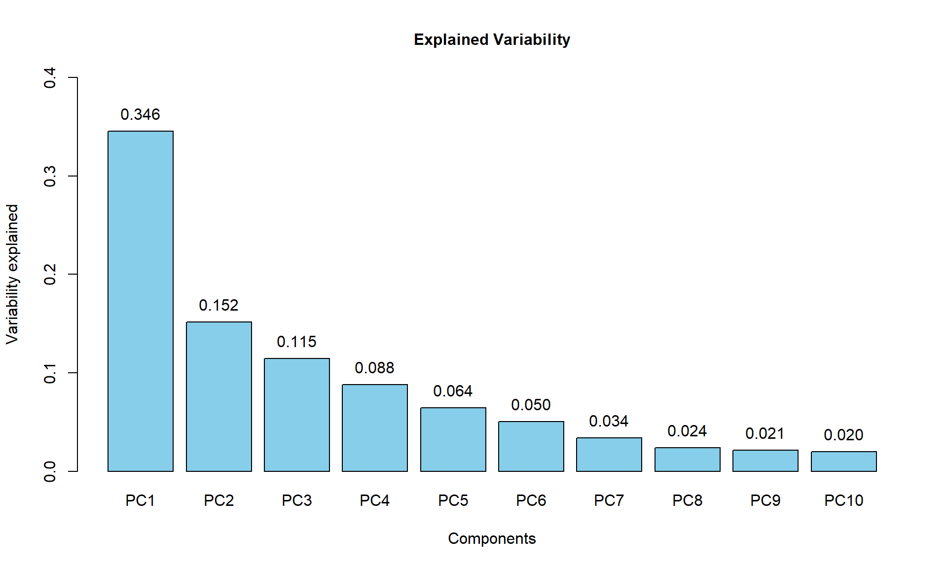

or using a package::function factoextra::fviz_eig() (try it, if you wish). factoextra::fviz_eig(PC, addlabels = TRUE, main="Explained Variability (fviz_eig)")

Another powerful package: PCAtools

## please install: PCAtools and ggalt

#install.packages("BiocManager")
#BiocManager::install("PCAtools")
#install.packages("ggalt")

library(PCAtools)

p = pca(mRNA$X, removeVar = 0, metadata = mRNA$meta)
biplot(p, colby="time", title="Principal Component Analysis", legendPosition = "bottom", showLoadings  = TRUE,encircle=TRUE)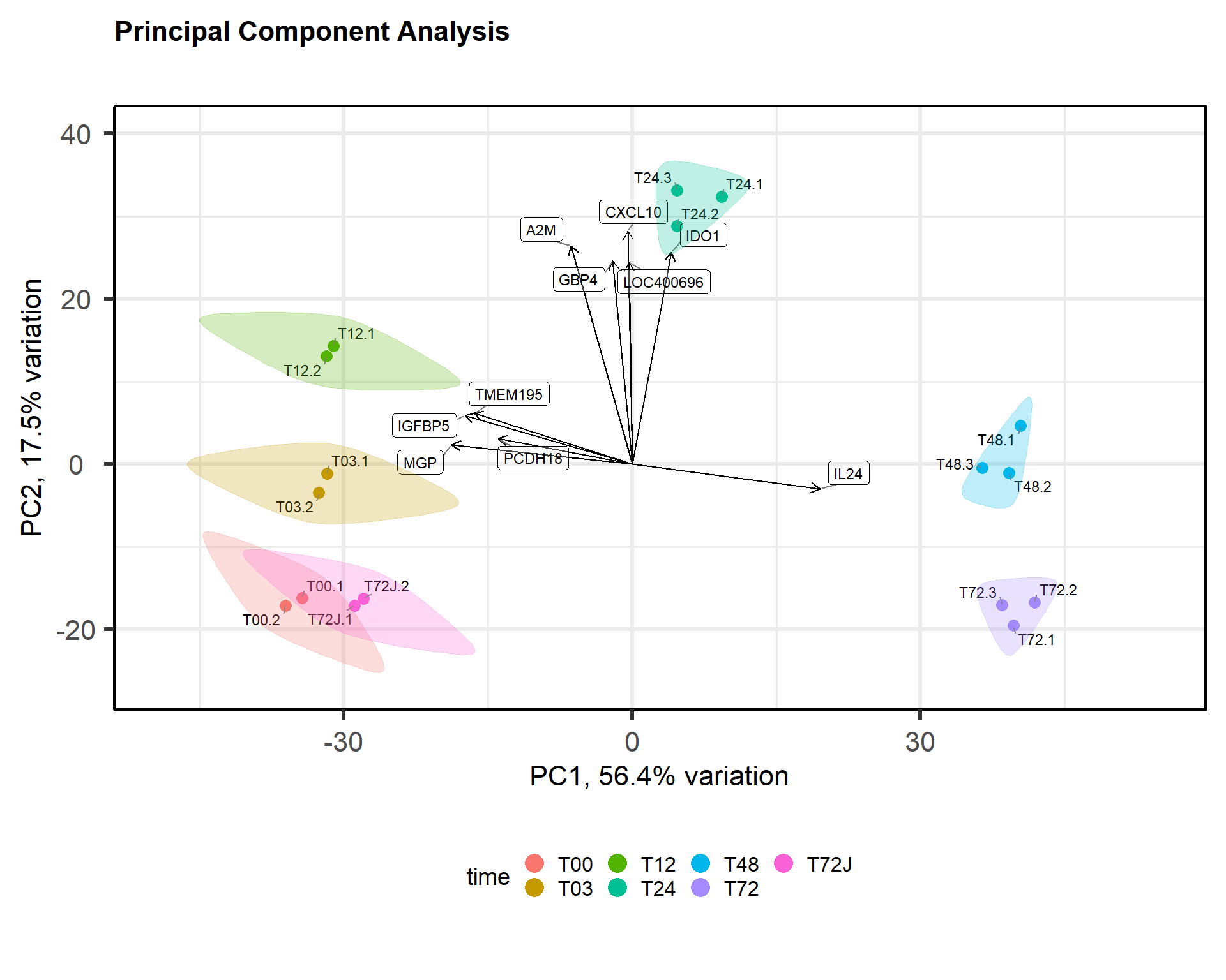

screeplot(p, axisLabSize = 8, titleLabSize = 22)

3.2.2 PCA of genes in the space of samples

We can also use PCA to see similarity between features. Let’s also highlight marker genes.

size = 0.5 + apply(mRNA$X,1,mean)/6

## Log intensities
plotPCA( t(mRNA$X),
         col="#00AA0022", 
         cex=size, 
         main = "PCA for genes (sample space)")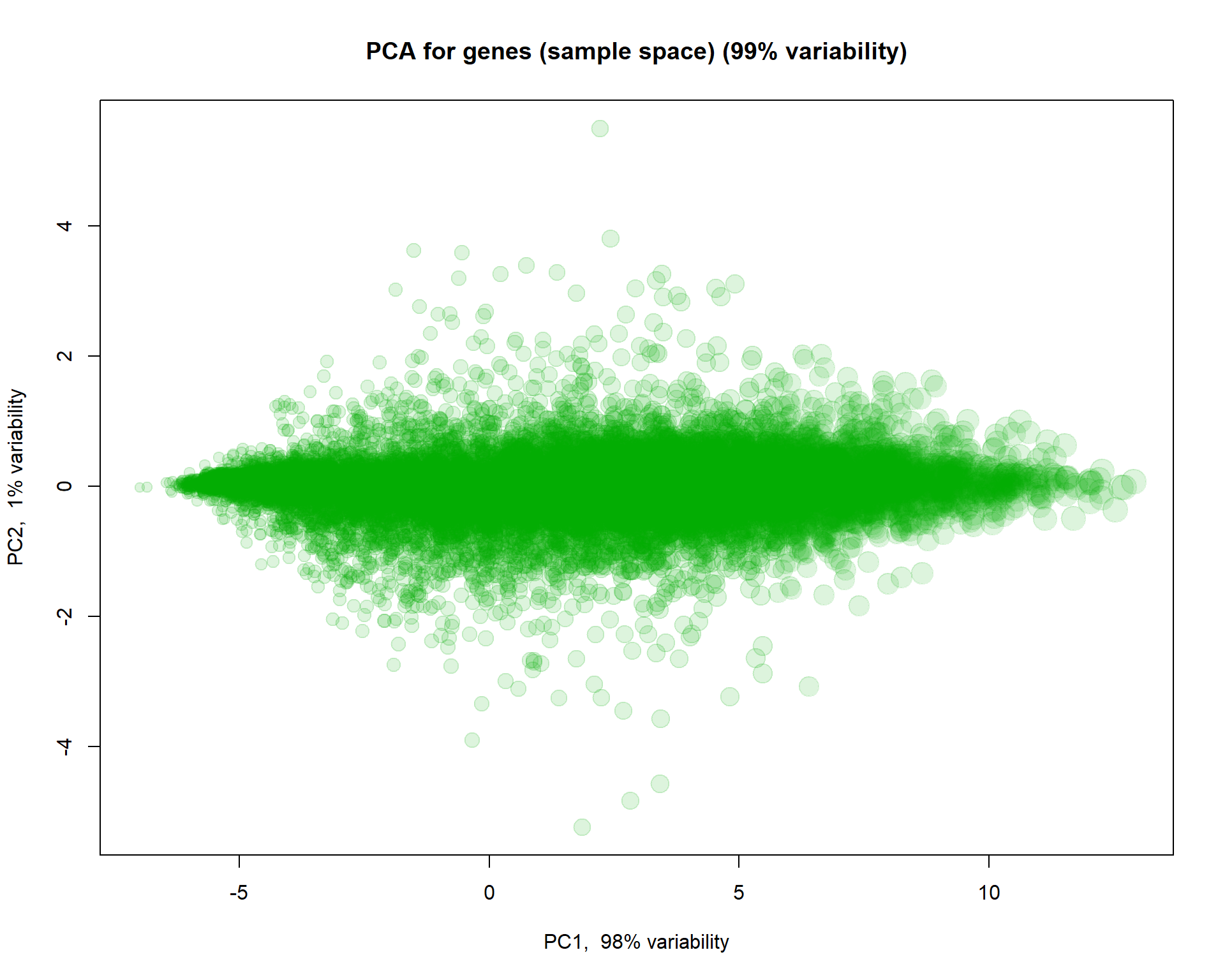

## you can check behaviour of with treatment "VEGFA","IRF1","SOX5

This is not too informative, as 98% of variability is related to overall gene expression. Let’s normalize genes (each gene will have mean = 0, st.dev = 0 over samples).

## Let's scale expression
Z = mRNA$X
Z[,] = t(scale(t(Z)))

PC2 = prcomp(Z,scale=TRUE)
plotPCA(t(Z),pc = PC2,col="#00AA0011", cex=size, main = "Standardized expression (per gene)")

## select 3 genes and show them
genes = c(which.min(PC2$x[,1]),which.max(PC2$x[,1]),which.min(abs(PC2$x[,1]-2) * abs(PC2$x[,2]-1)))
text(PC2$x[genes,1],PC2$x[genes,2],names(genes),col=1,pch=19,font=2)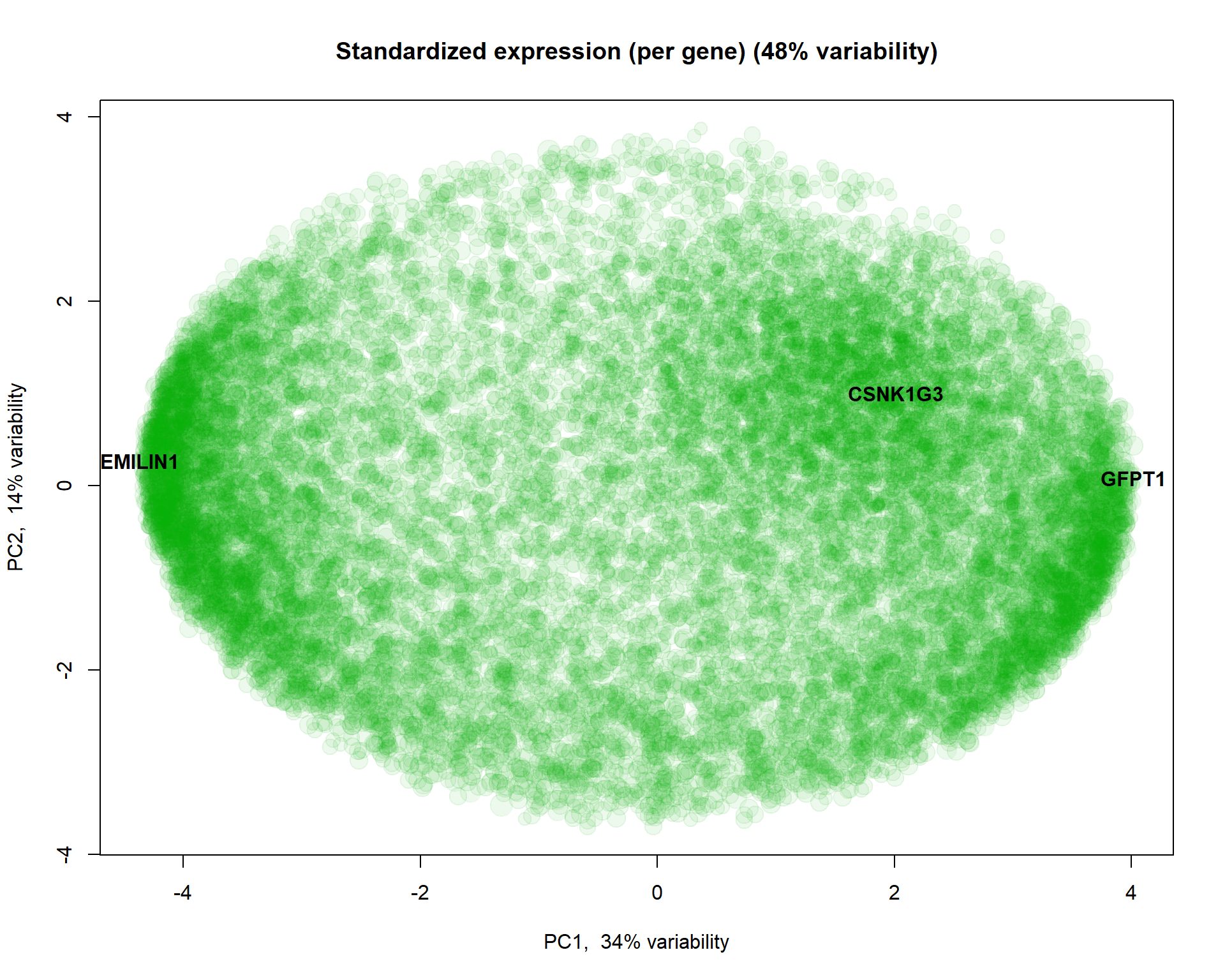

I selected here 3 genes for a detailed investigation:

## behaviour with treatment
par(mfcol=c(1,3))
boxplot(mRNA$X[genes[1],]~mRNA$meta$time, main = names(genes)[1], col = 1:nlevels(mRNA$meta$time))
boxplot(mRNA$X[genes[2],]~mRNA$meta$time, main = names(genes)[2], col = 1:nlevels(mRNA$meta$time))
boxplot(mRNA$X[genes[3],]~mRNA$meta$time, main = names(genes)[3], col = 1:nlevels(mRNA$meta$time))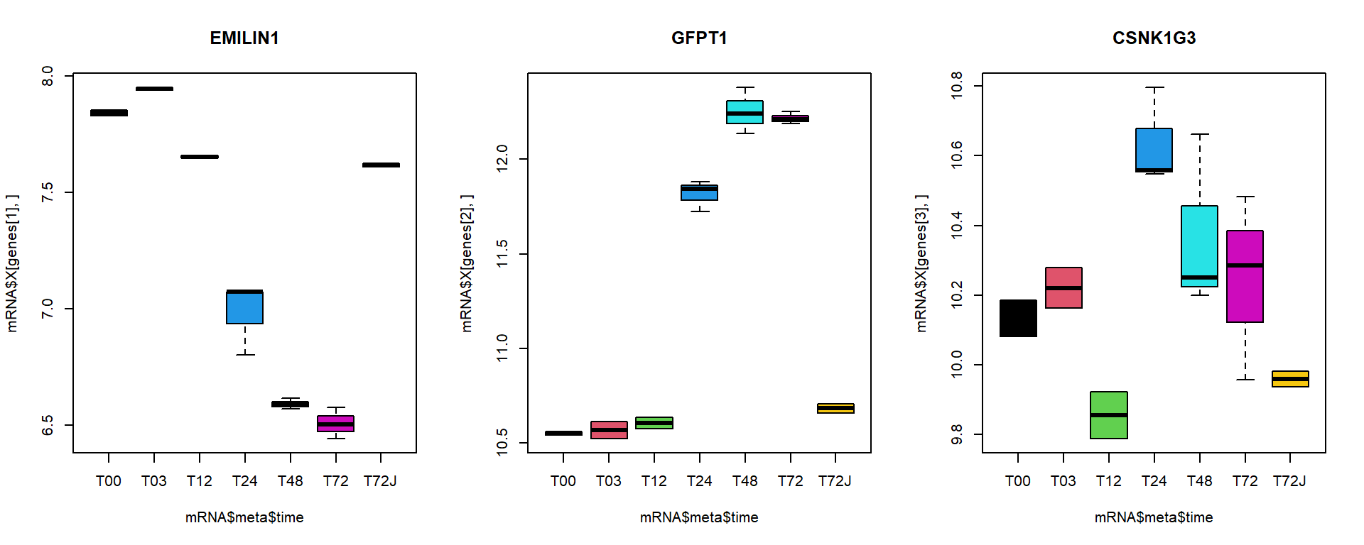

3.3. MDS

Classical MDS can be performed using cmdscale() function

## calculate euclidean distances
d = dist(t(mRNA$X)) 

## fit distances in 2D space to distances in multidimensional space
MDS = cmdscale(d,k=2) 
str(MDS)

##  num [1:17, 1:2] -34.4 -36.1 -31.8 -32.6 -31.1 ...
##  - attr(*, "dimnames")=List of 2
##   ..$ : chr [1:17] "T00.1" "T00.2" "T03.1" "T03.2" ...
##   ..$ : NULL

plot(MDS[,1],MDS[,2],col=as.integer(mRNA$meta$time),pch=19, main="MDS plot",cex =2)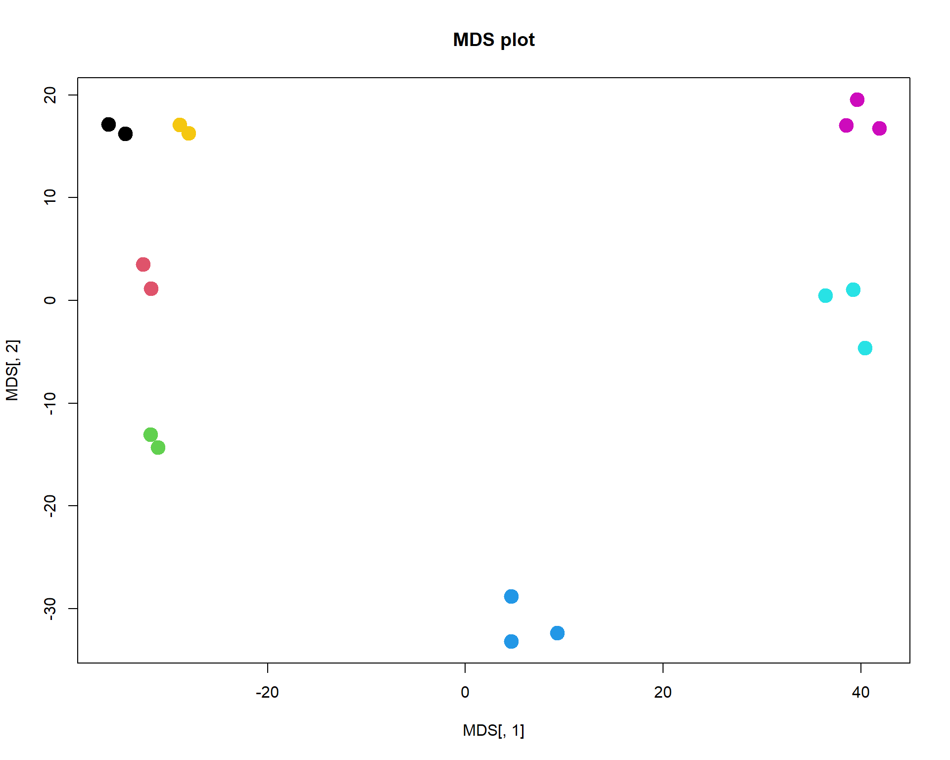

As you can see, it is very close to PCA results. But it requires much more computational power, when working with large number of objects. It may outperform PCA in a special case, when variance captured by 1st, 2nd and 3rd components is similar. Or when you need a special type of distance.

3.4. ICA

ICA, similar to PCA, but tries to extract statistically independent signals. This signals are correlated to biological processes more often than for PCA. But to see ICA power we need a lot of data. Here results will be similar to MDS.

source("http://r.modas.lu/LibICA.r")

## [1] "----------------------------------------------------------------"
## [1] "libML: Machine learning library"
## [1] "Needed:"
## [1] "randomForest" "e1071"       
## [1] "Absent:"
## character(0)
## [1] "----------------------------------------------------------------"
## [1] "consICA: Checking required packages and installing missing ones"
## [1] "Needed:"
##  [1] "fastICA"      "sm"           "vioplot"      "pheatmap"     "gplots"      
##  [6] "foreach"      "survival"     "topGO"        "org.Hs.eg.db" "org.Mm.eg.db"
## [11] "doSNOW"      
## [1] "Absent:"
## character(0)

IC = runICA(mRNA$X,ntry=100,ncomp=3,ncores=2)

## *** Starting parallel calculation on 2 core(s)...
## *** System: windows 
## *** 3 components, 100 runs, 20141 features, 17 samples.
## *** Start time: 2022-10-10 00:13:41 
## *** Done! 
## *** End time: 2022-10-10 00:13:48 
## Time difference of 7.351828 secs
## Calculate ||X-SxM|| and r2 between component weights
## Correlate rows of S between tries
## Build consensus ICA
## Analyse stability

par(mfcol=c(1,3))
plot(IC$M[1,],IC$M[2,],pch=19,col=as.integer(mRNA$meta$time),cex=2,main="IC1-IC2")
plot(IC$M[1,],IC$M[3,],pch=19,col=as.integer(mRNA$meta$time),cex=2,main="IC1-IC3")
plot(IC$M[2,],IC$M[3,],pch=19,col=as.integer(mRNA$meta$time),cex=2,main="IC2-IC3")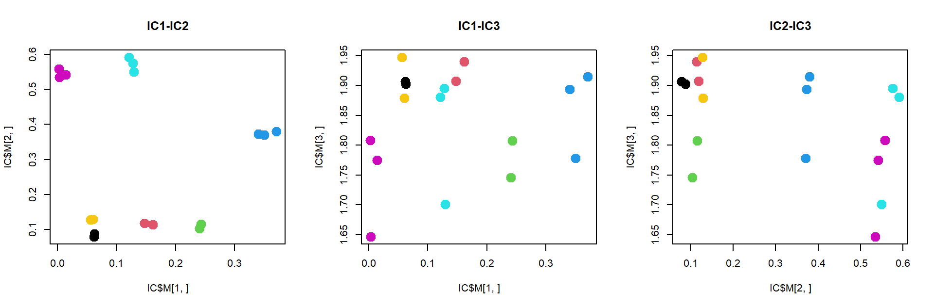

3.5. t-SNE

Unlike PCA, t-SNE shows not differences, but rather similarities. Similar objects should be located together. The method does not care about distant objects. The distance is weighted by Student (t) distribution (similar to Gaussian).

Let’s use Rtsne package. Please note, that when your dataset is large, it is recommended to do PCA first before sending your data to t-SNE. In Rtsne they use so called “Barnes-Hut implementation” - faster but approximate.

#install.packages("Rtsne")
library(Rtsne)
## plot samples (not interesting)
TS1 = Rtsne(t(mRNA$X),perplexity=3,max_iter=2000)$Y
plot(TS1[,1],TS1[,2],col=as.integer(mRNA$meta$time),pch=19,cex=2, main="tSNE for samples (reducing gene space)")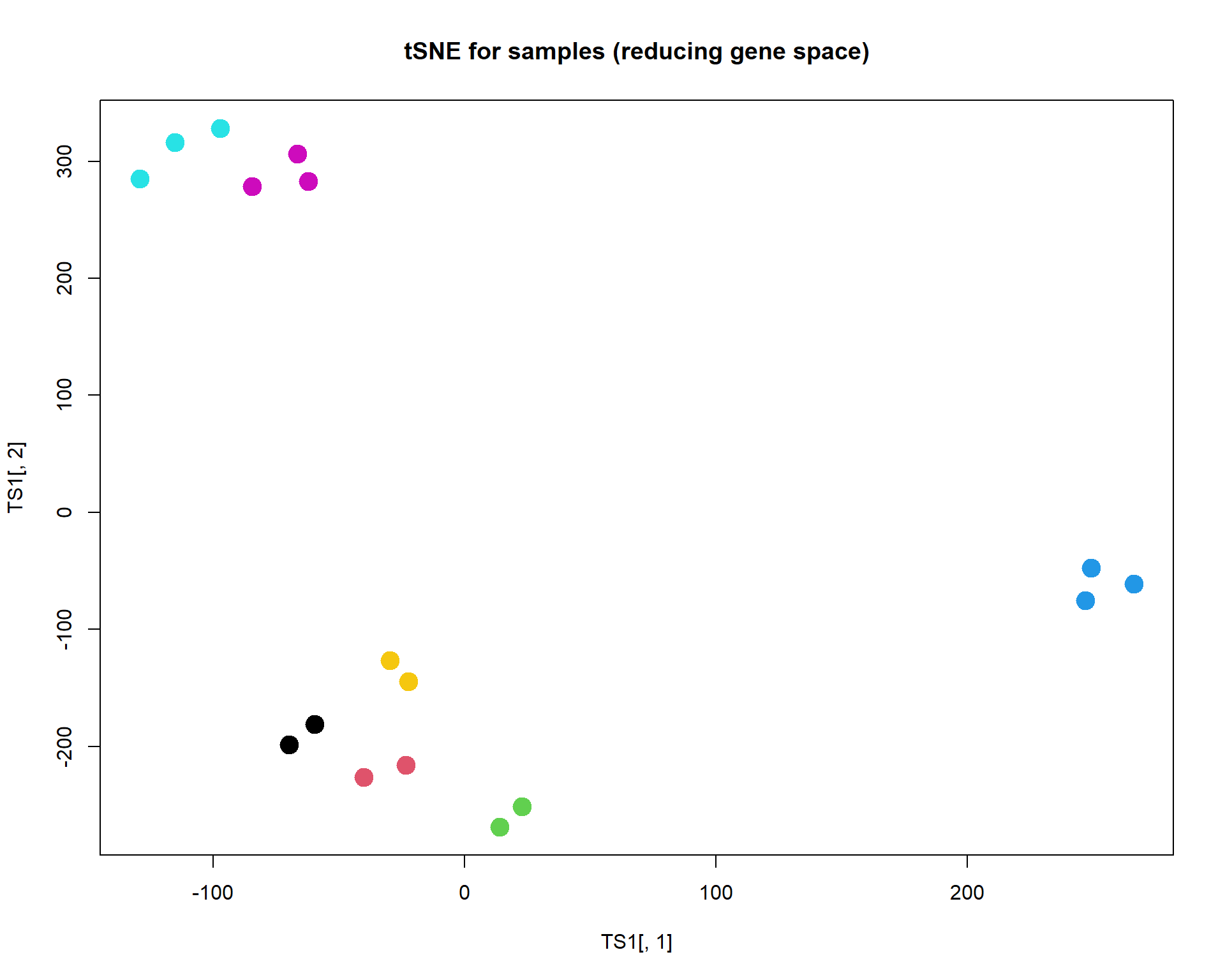

## plot features
TS2x = Rtsne(mRNA$X,perplexity=20,max_iter=1000,check_duplicates = FALSE )$Y
plot(TS2x[,1],TS2x[,2],col="#00AA0033",pch=19,cex=size, main="tSNE for genes (original)")
text(TS2x[genes,1],TS2x[genes,2],names(genes),col=1,pch=19,font=2)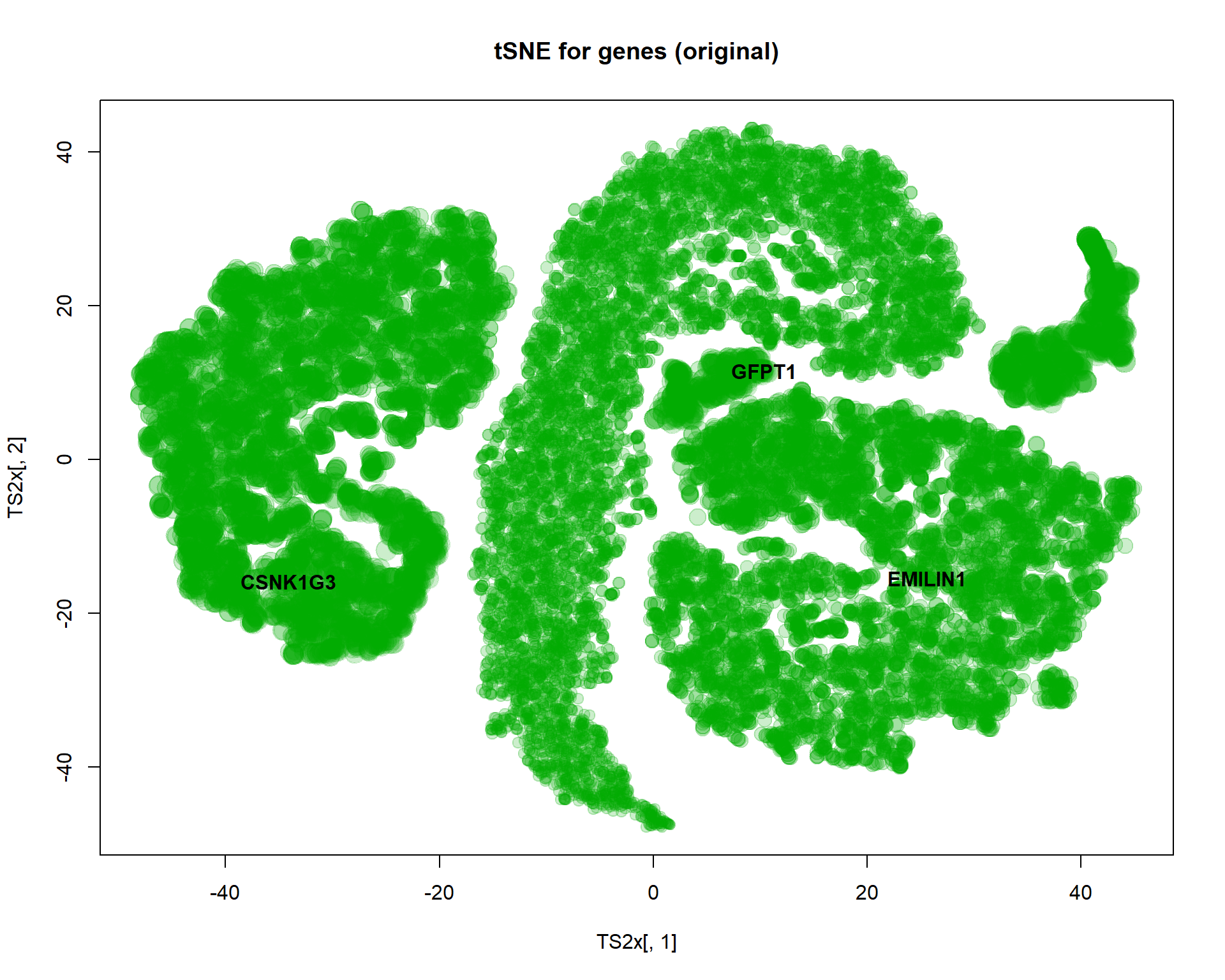

## same for scaled features (Z was calculated earlier)
TS2z = Rtsne(Z,perplexity=50,max_iter=1000,check_duplicates = FALSE)$Y
plot(TS2z[,1],TS2z[,2],col="#00AA0033",pch=19,cex=size, main="tSNE for genes (standardized genes)")
text(TS2z[genes,1],TS2z[genes,2],names(genes),col=1,pch=19,font=2)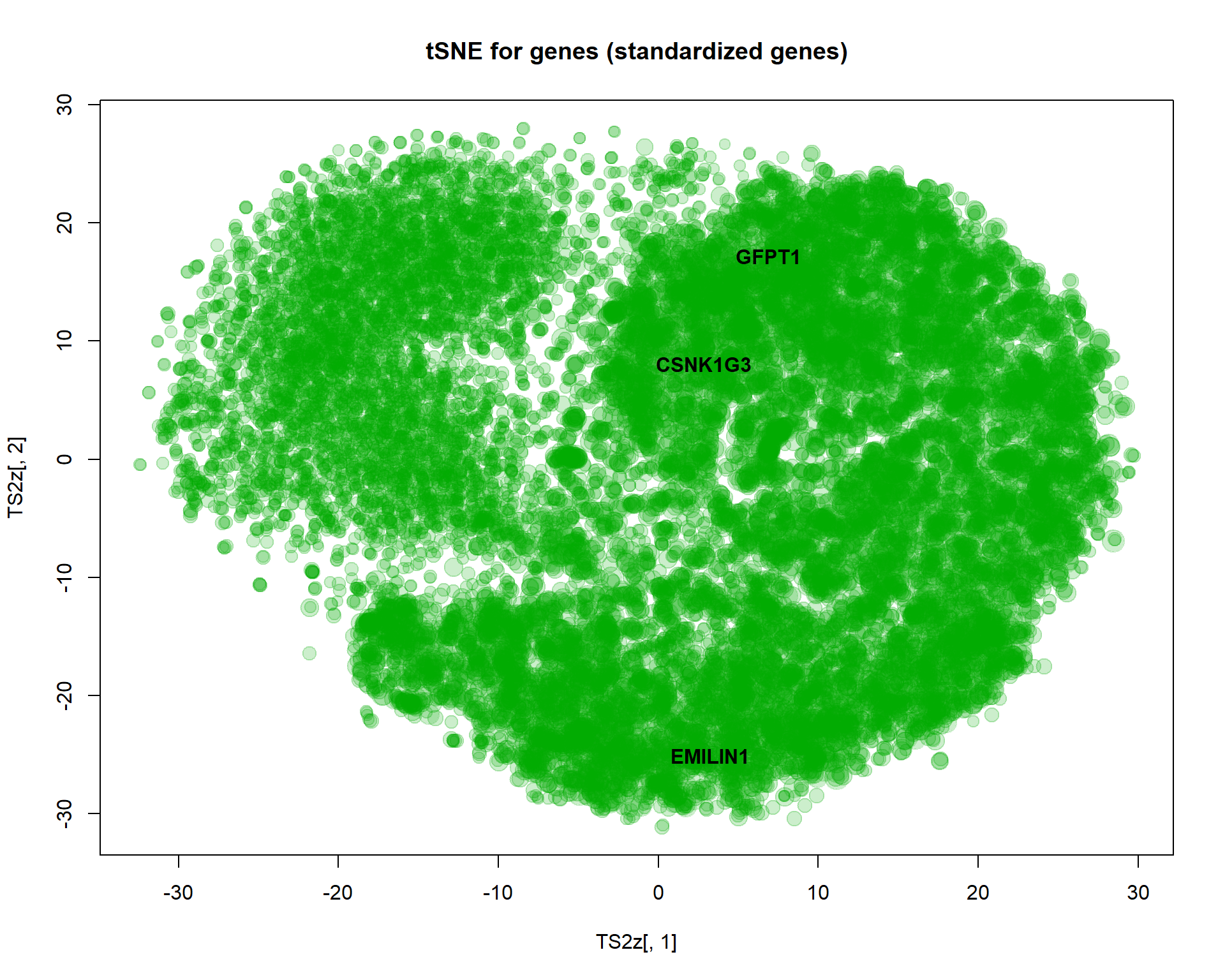

There is another package - tsne. It is slower, but in some cases more precise. If “precise” can be used for describing t-SNE ;)

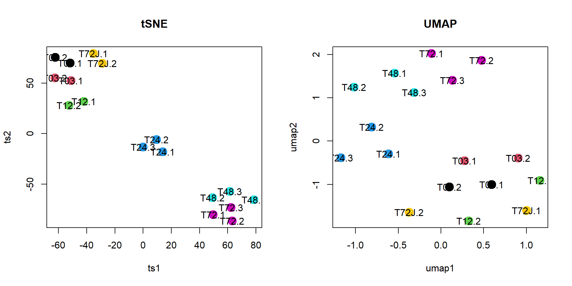
Exercises

Build PCA for miR data. Access to the data - miR$X. Sample annotation - miR$meta

prcomp() and t(), plotPCA()

Build PCA for mice from Mice data and identify ourliers. Use the data frame without 3 first columns: Mice[,-(1:3)]

prcomp() and text(); or plotPCA() and t()

Build MDS for miR data.

dist(), t(), cmdscale()

Build tSNE for iris data. Use all columns except 5th for calculation, and 5th - for coloring.

Rtsne()

Prev Home Next

By Petr Nazarov