4. Clustering

You should have loaded the following data:

miR & mRNA - microRNA and mRNA profiles of A375 cell line after stimulation with IFNg (adapted from [Nazarov et al, Nucleic Acid Research, 2013])

If not, please load:

## load the script from Internet
source("http://r.modas.lu/readAMD.r")

## miRNA data
miR = readAMD("http://edu.modas.lu/data/txt/mirna_ifng.amd.txt",stringsAsFactors = TRUE)

## mRNA data
mRNA = readAMD("http://edu.modas.lu/data/txt/mrna_ifng.amd.txt",
               stringsAsFactors = TRUE,
               index.column="GeneSymbol",
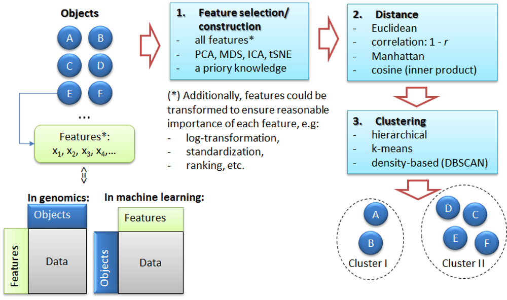
               sum.func="mean")

4.1. The task of clustering

The task of clustering: (1) feature selection, (2) distance estimation, (3) unsupervised grouping - clustering

4.2. k-Means clustering

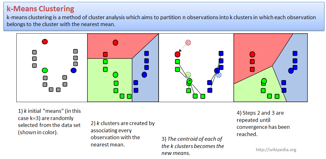
k-Means clustering - a simple and robust approach.

Let us try to cluster standard iris dataset.We will use PCA to present samples in 2D space, and next cluster with a standard kmeans function.

centers - number of clusters (k);
to make analysis more reproducible - increase nstart

## define shape - actual species
pch = c(15,16,17)[as.integer(iris$Species)]

PC = prcomp(iris[,-5],scale=TRUE) 
plot(PC$x[,"PC1"],PC$x[,"PC2"],col=as.integer(iris$Species),pch=pch,cex=2, main="Flowers in PC-space: Species as Ground Truth")

## clustering -> 3 clusters
str(kmeans(iris[,-5],centers=3,nstart=10))

## List of 9
##  $ cluster     : int [1:150] 1 1 1 1 1 1 1 1 1 1 ...
##  $ centers     : num [1:3, 1:4] 5.01 6.85 5.9 3.43 3.07 ...
##   ..- attr(*, "dimnames")=List of 2
##   .. ..$ : chr [1:3] "1" "2" "3"
##   .. ..$ : chr [1:4] "Sepal.Length" "Sepal.Width" "Petal.Length" "Petal.Width"
##  $ totss       : num 681
##  $ withinss    : num [1:3] 15.2 23.9 39.8
##  $ tot.withinss: num 78.9
##  $ betweenss   : num 603
##  $ size        : int [1:3] 50 38 62
##  $ iter        : int 2
##  $ ifault      : int 0
##  - attr(*, "class")= chr "kmeans"

cl = kmeans(iris[,-5],centers=3,nstart=10)$cluster
plot(PC$x[,"PC1"],PC$x[,"PC2"],col=cl+1,pch=pch,cex=2, main="Flowers in PC-space: k-means, k=3")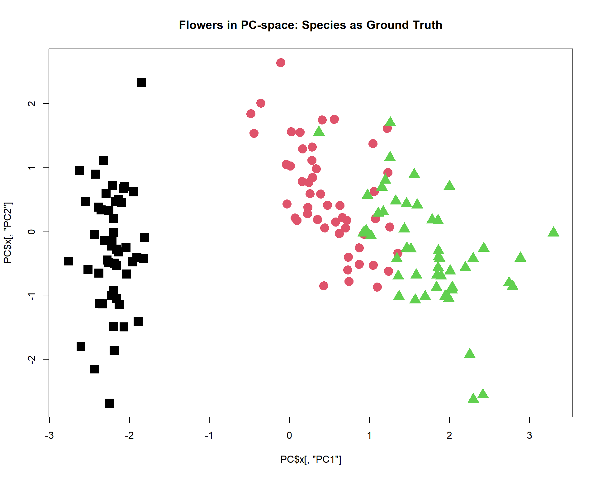

Try to change number of clusters.

par(mfcol=c(1,2))
cl = kmeans(iris[,-5],centers=2,nstart=10)$cluster
plot(PC$x[,"PC1"],PC$x[,"PC2"],col=cl+1,pch=pch,cex=1.2, main="Flowers in PC-space: k-means, k=2")
cl = kmeans(iris[,-5],centers=4,nstart=10)$cluster
plot(PC$x[,"PC1"],PC$x[,"PC2"],col=cl+1,pch=pch,cex=1.2, main="Flowers in PC-space: k-means, k=4")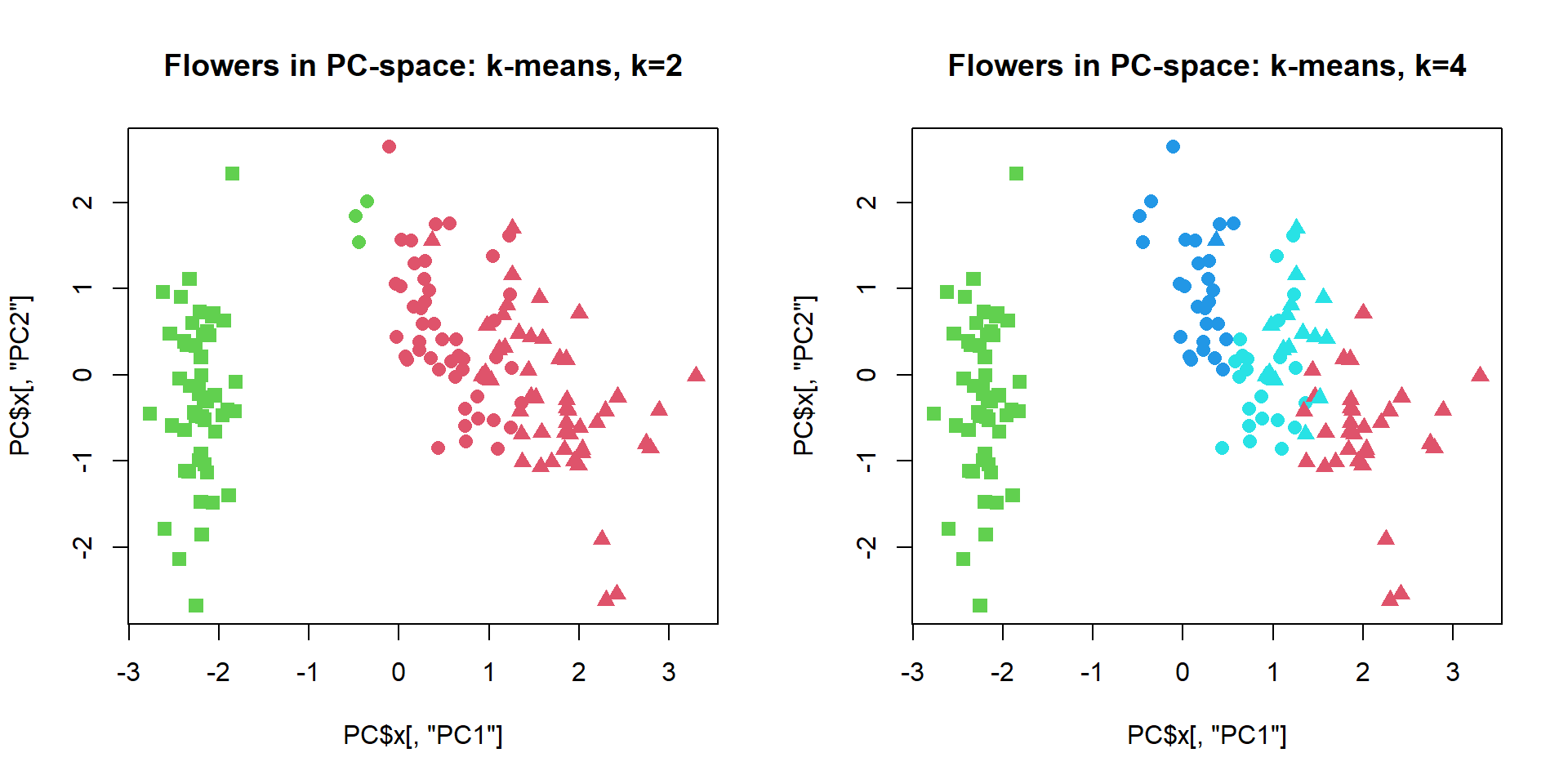

We can also cluster features - usually not very interesting with k-means. Working with

source("http://r.modas.lu/plotPCA.r")

## Let's scale expression
Z = mRNA$X
Z[,] = t(scale(t(Z)))

PC2 = prcomp(Z,scale=TRUE)
genecl = kmeans(Z,centers=4,nstart=10)$cluster

par(mfcol=c(1,2))
plotPCA(t(Z),pc = PC2,col=genecl+1, cex=0.5, main = "Stand.expr., 4 cl.")
plotPCA(t(Z),pc = PC2, ipc=(3:4), col=genecl+1, cex=0.5, main = "Stand.expr., 4 cl.")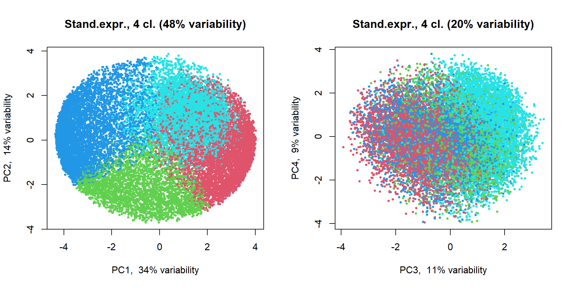

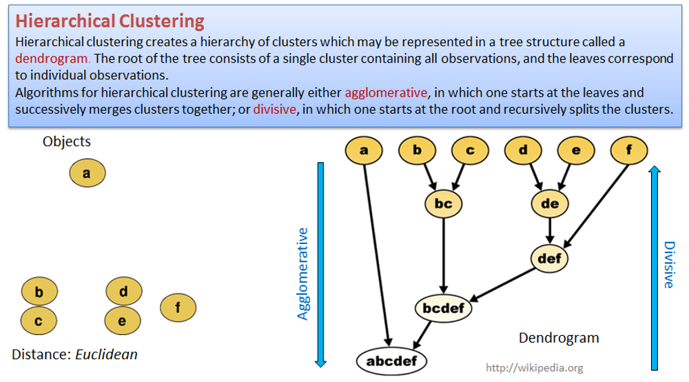
4.3. Hierarchical clustering

Hierarchical clustering - more flexible but less robust approach

## clustering of the samples
hc = hclust(dist(iris[,-5]))
plot(hc,cex=0.6)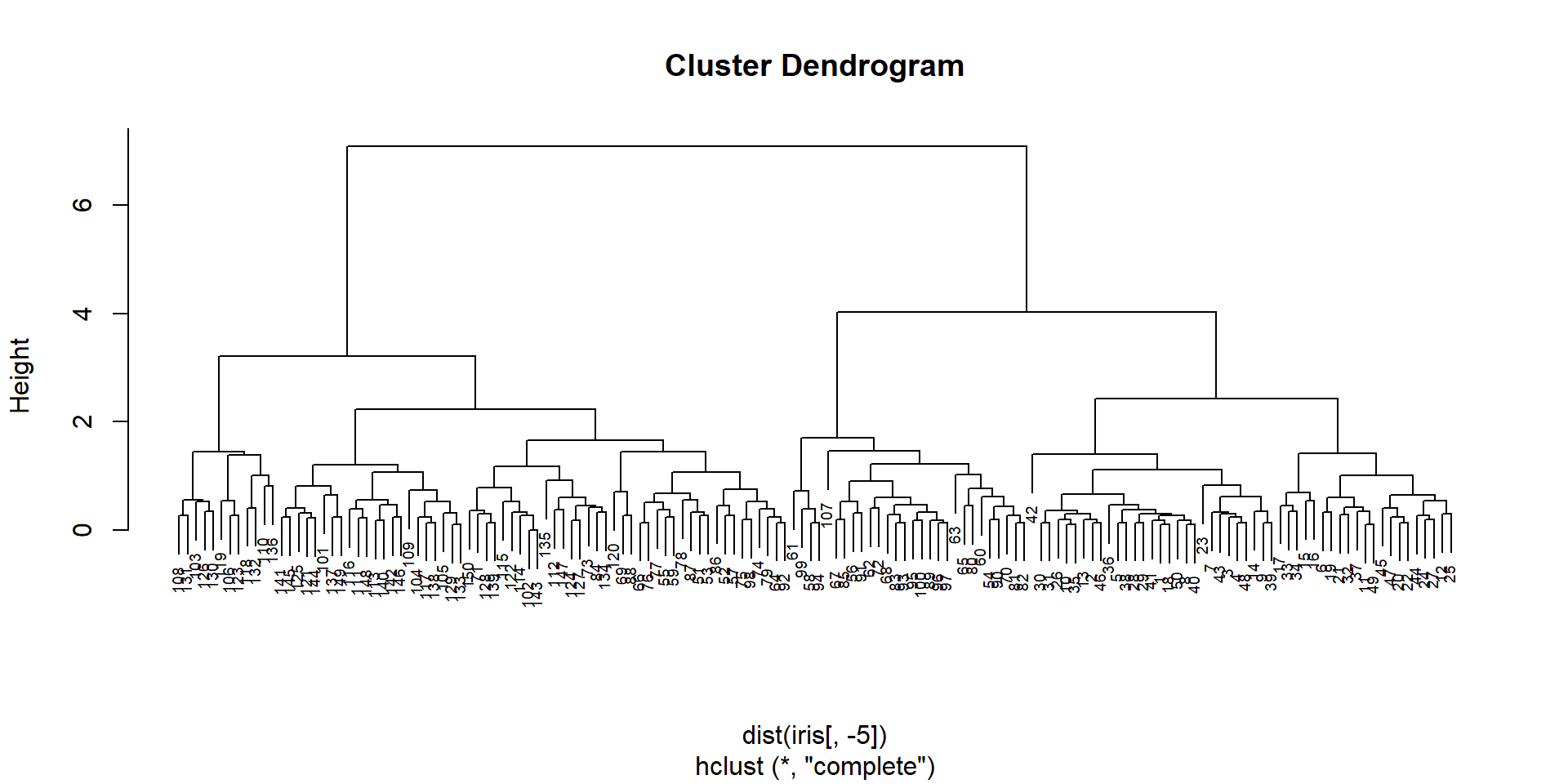

We need to “cut the tree” in order to get clusting:

## "cut the tree" to get defined clusters
cl = cutree(hc,k=3)
plot(PC$x[,"PC1"],PC$x[,"PC2"],col=cl+1,pch=pch,cex=2, main="Flowers, hclust with 3 cl.")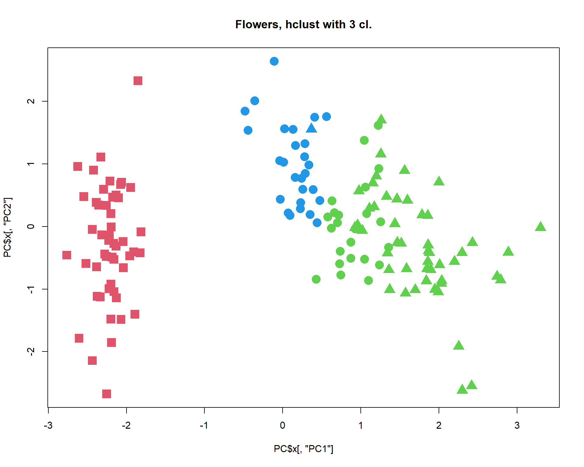

## play with k...

Let’s play with number of clusters

par(mfcol=c(1,2))
cl = cutree(hc,k=2)
plot(PC$x[,"PC1"],PC$x[,"PC2"],col=cl+1,pch=pch,cex=1.2, main="Flowers, hclust with 2 cl.")
cl = cutree(hc,k=4)
plot(PC$x[,"PC1"],PC$x[,"PC2"],col=cl+1,pch=pch,cex=1.2, main="Flowers, hclust with 4 cl.")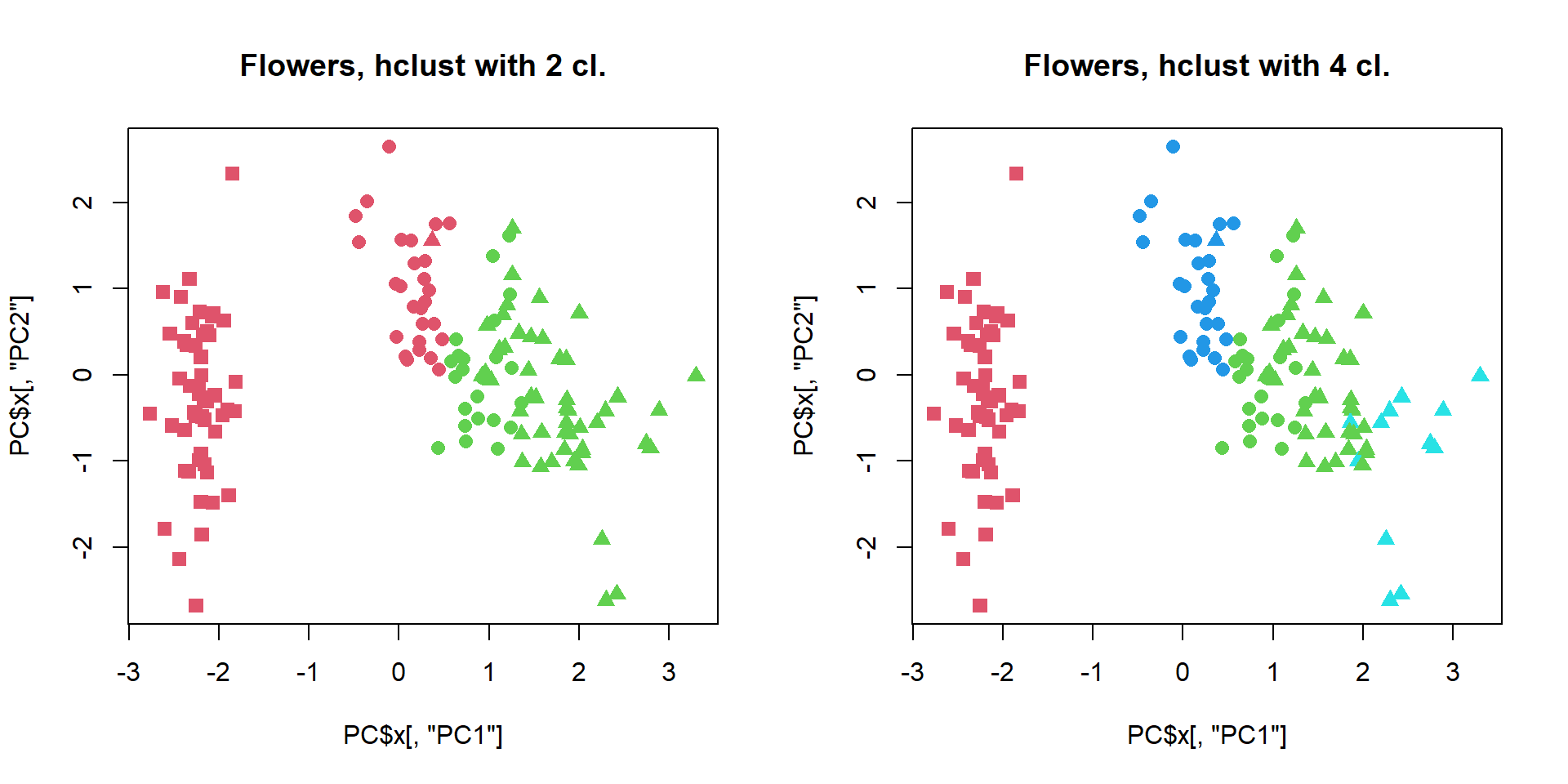

Hierarchical clustering allows more freedom (same tree can be cut at diferent depth), but it is not robust - removing one sample will change clustering! Usually people apply consensus hierarchical clustering to get defined and robust clusters.

Let’s install ant test package ConsensusClusterPlus. Instead of iris, we will test it on mRNA data

#BiocManager::install("ConsensusClusterPlus")
library(ConsensusClusterPlus)

## select the most variable genes
thr = quantile(apply(mRNA$X,1,sd),0.95) ## thr <- st.dev. for 5% the most variable genes
ikeep = apply(mRNA$X,1,sd)> thr ## index of genes with st.dev > thr 
table(ikeep) ## check numbers

## ikeep
## FALSE  TRUE 
## 19134  1007

## calculate standardized gene expression for the most variable genes
Z = mRNA$X[ikeep,]
Z[] = t(scale(t(Z)))
PC = prcomp(t(Z))

## you can skip this line! 
   setwd("d:/data/r")
## cons clustering of the samples
hc = ConsensusClusterPlus(t(Z),
                          maxK=6,
                          reps=100,
                          pItem=0.8,
                          pFeature=1, 
                          title="CC_hc",
                          clusterAlg="hc",
                          distance="euclidean",
                          seed=1234567890,
                          plot="png")
## get clusters
cl=hc[[5]]$consensusClass
## plot
plotPCA(t(Z),col = cl+1)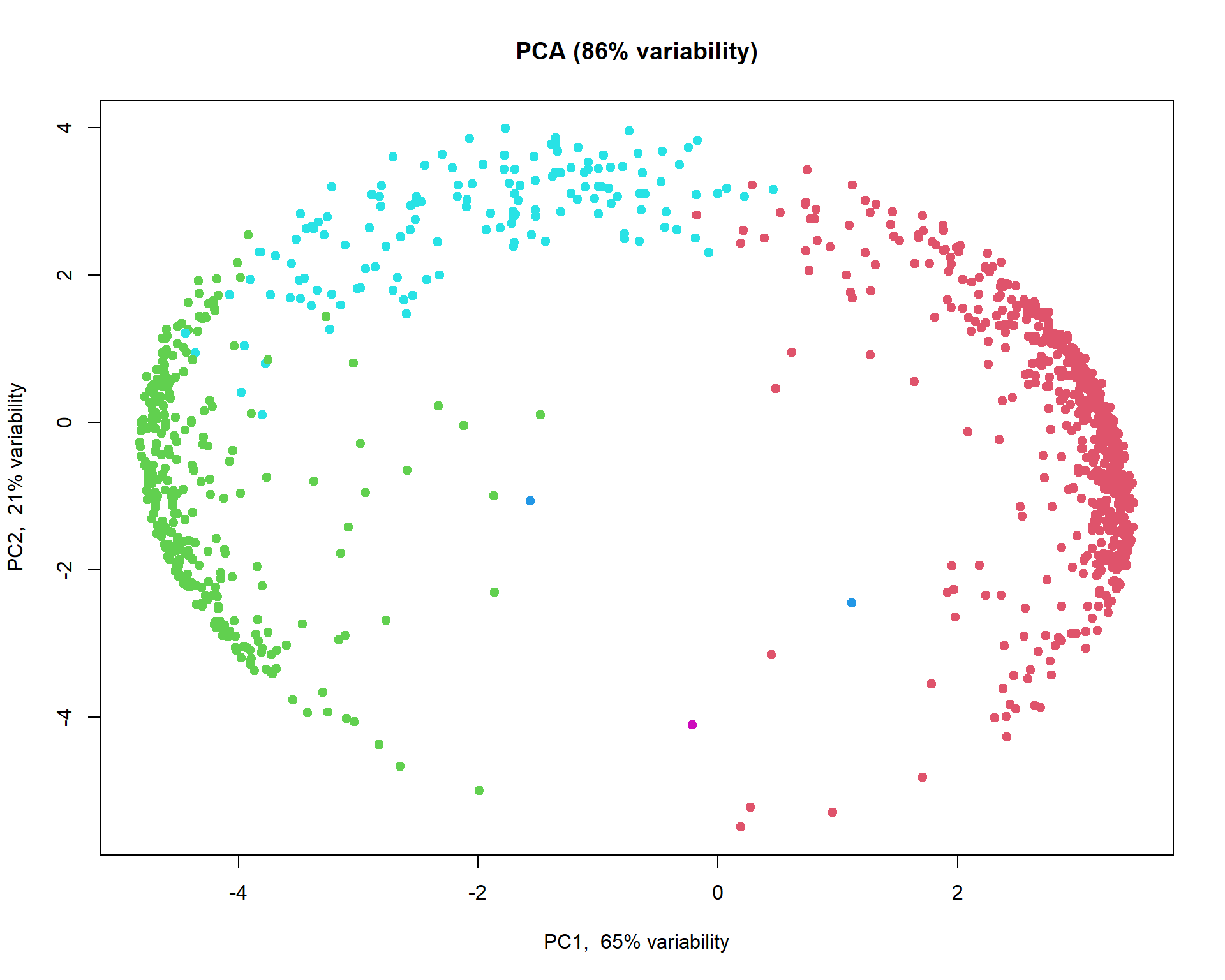

Now we can calculate and plot mean expression for the clusters

## select 3 larger clusters
summary(as.factor(cl))

##   1   2   3   4   5 
## 560 302   2 142   1

icl = order(summary(as.factor(cl)),decreasing=TRUE)[1:3]

## calculate mean profile over standardized genes for each cluster
z1 = apply(Z[cl == icl[1],],2,mean)
z2 = apply(Z[cl == icl[2],],2,mean)
z3 = apply(Z[cl == icl[3],],2,mean)

## plot results
par(mfcol = c(1,3))
boxplot(z1~mRNA$meta$time,las=2,col=1:nlevels(mRNA$meta$time), main="Mean expression in cl.1")
boxplot(z2~mRNA$meta$time,las=2,col=1:nlevels(mRNA$meta$time), main="Mean expression in cl.2")
boxplot(z3~mRNA$meta$time,las=2,col=1:nlevels(mRNA$meta$time), main="Mean expression in cl.3")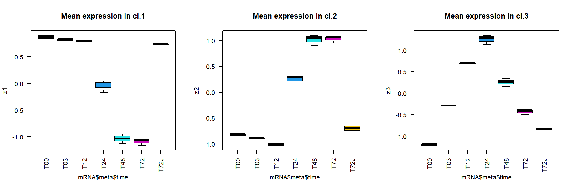

4.5. Number of clusters

Note: despite many methods exist, from my experience - there in no magic pill! Let’s calculate number of clusters for the most variable mRNA in IFNg experiment. We will use package factoextra. The standard methods are:

Silhouette - how similar each object is to other object of his cluster in comparison to other objects
WSS or WCSS - within cluster sum of squares
Gap statistics - gap statistics of Tibshirani

#install.packages("factoextra")
library(factoextra)
## this can be slow.. try it:
fviz_nbclust(Z, kmeans, method = "silhouette", print.summary =FALSE,verbose =FALSE)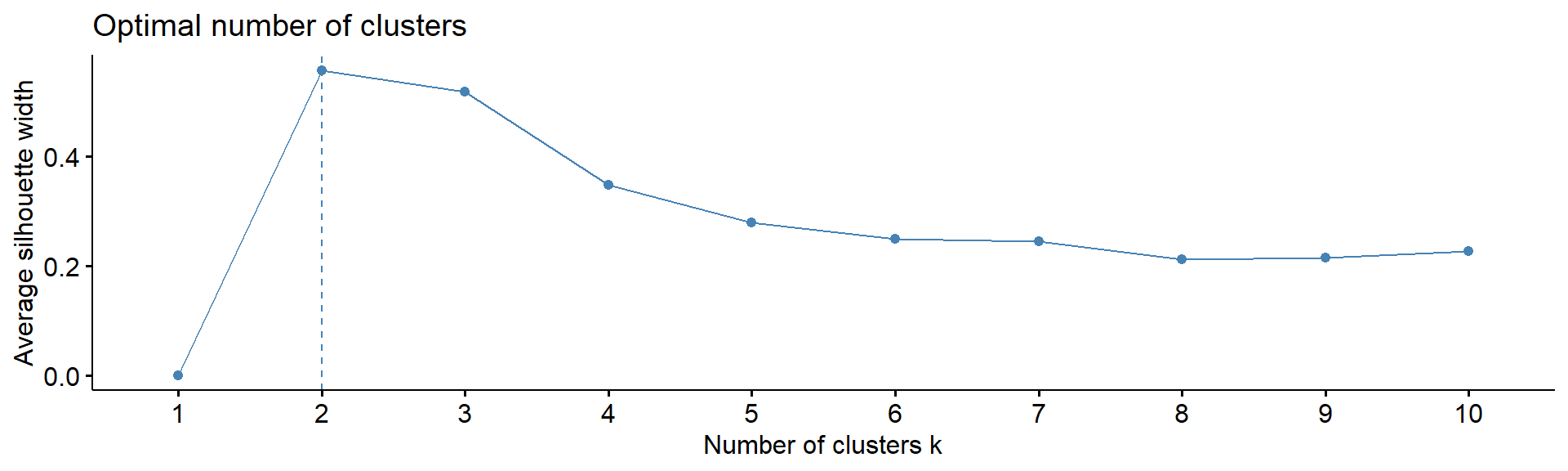

fviz_nbclust(Z, kmeans, method = "wss", print.summary =FALSE,verbose =FALSE)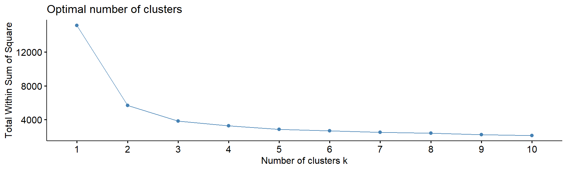

fviz_nbclust(Z, kmeans, method = "gap_stat", print.summary =FALSE,verbose =FALSE)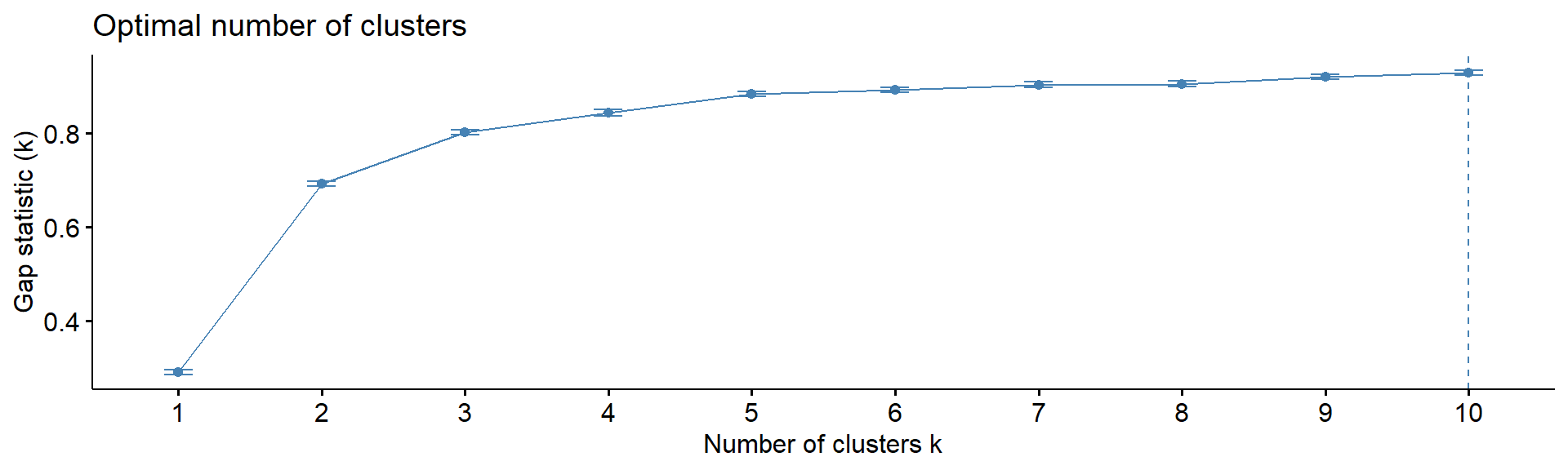

4.5. Heatmaps

One of the most used methods for visualizing omics data is heatmap. Here we will use heatmaps from the package pheatmap.

#install.packages("pheatmap")
library(pheatmap)
## let's use previously defined markers
pheatmap(Z, 
         annotation_col = mRNA$meta,
         fontsize_row = 2)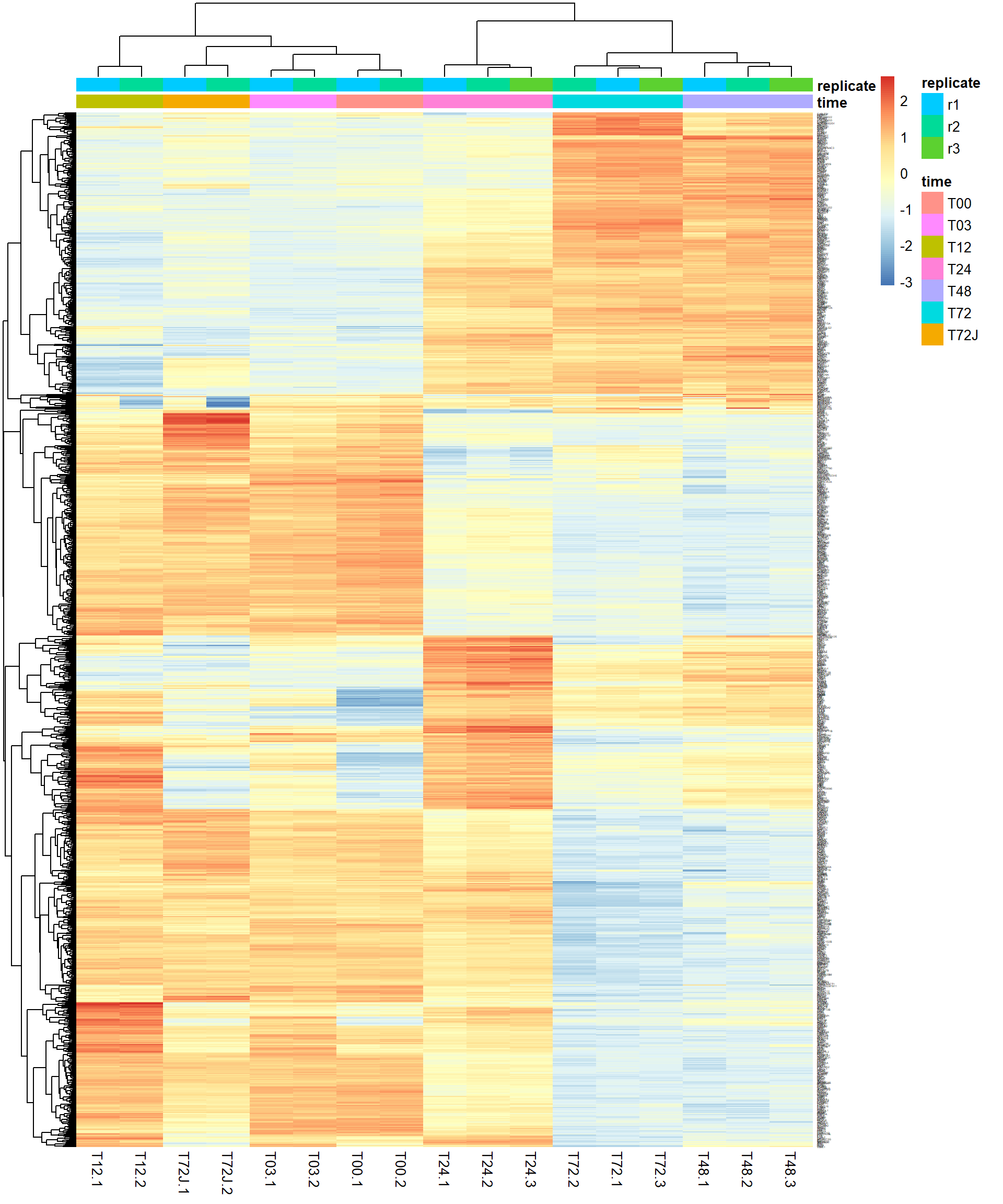

You could also try standard heatmap() and gplots::hearmap.2(). They give more control over distance measures and clustering.

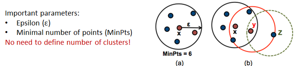
4.6. Density-based clustering

Working with

DBScan theory

Comparison

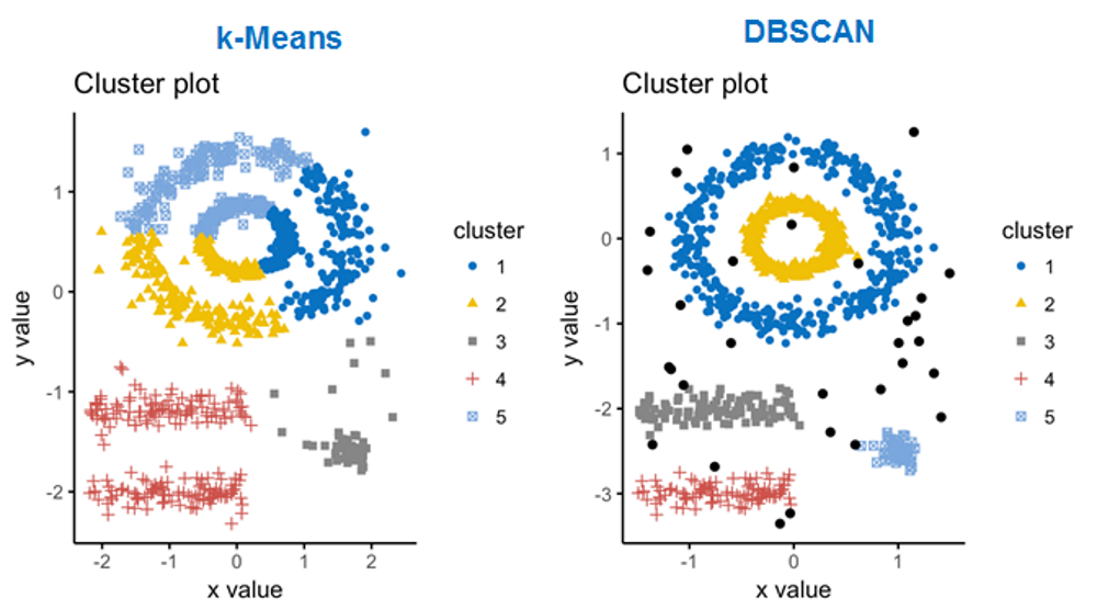
Let’s read and visualize pre-analyzed dataset (GSE81547) - single-cell experiment on samples taken from pancreas. Data were downloaded, PCA-transformed and t-SNE was calculated on the first 100 components.

Panc = read.table("http://edu.modas.lu/data/txt/tsne_normpancreas.txt",sep="\t",header=TRUE,row.names=1,as.is=FALSE)
str(Panc)

## 'data.frame':    2544 obs. of  7 variables:
##  $ individual        : Factor w/ 8 levels "DID_scRSq01",..: 4 4 4 4 4 4 4 4 4 4 ...
##  $ sex               : Factor w/ 2 levels "female","male": 2 2 2 2 2 2 2 2 2 2 ...
##  $ age               : int  21 21 21 21 21 21 21 21 21 21 ...
##  $ nreads            : int  447263 412082 167913 274448 323913 419043 600361 302079 262397 227087 ...
##  $ inferred.cell.type: Factor w/ 7 levels "acinar cell",..: 4 4 1 4 4 4 3 3 1 1 ...
##  $ tsne1             : num  33.2 32.6 20 31.8 31 ...
##  $ tsne2             : num  14 15.2 -51.6 14 16.4 ...

## color - inferred cell type
col = as.integer(Panc$inferred.cell.type)+1
## shape - individual
pch=13+as.integer(Panc$individual)
## plot & legend
plot(Panc$tsne1,Panc$tsne2,pch=pch,col=col,main="tSNE with Inferred Cell Type",xlim=c(-45,50))
legend("bottomright",levels(Panc$inferred.cell.type),pch=15,col=1+(1:nlevels(Panc$inferred.cell.type)))
legend("bottomleft","shape - patient")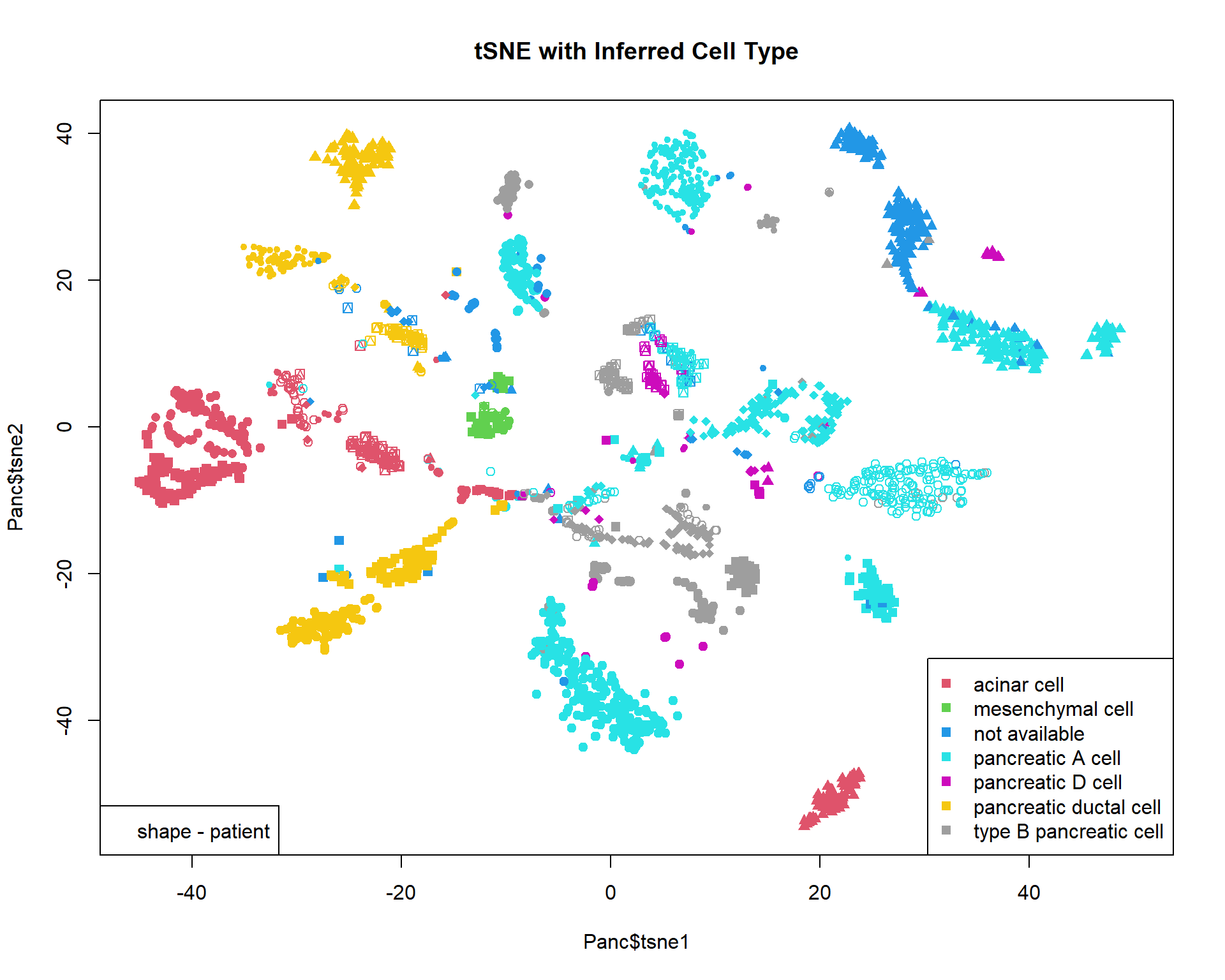

For single-cell data DBSCAN clustering is often used. We will work with package dbscan:

#install.packages("dbscan")
library(dbscan)

cl = dbscan(Panc[,c("tsne1","tsne2")],eps=2,minPts=10)$cluster
## cl==0 means no cluster - grey. Otherwise use color from rainbow()
col=c("#00000033",rainbow(max(cl),alpha=0.5))[cl+1]

plot(Panc$tsne1,Panc$tsne2,pch=19,col=col,main="tSNE Clusterng with DBSCAN")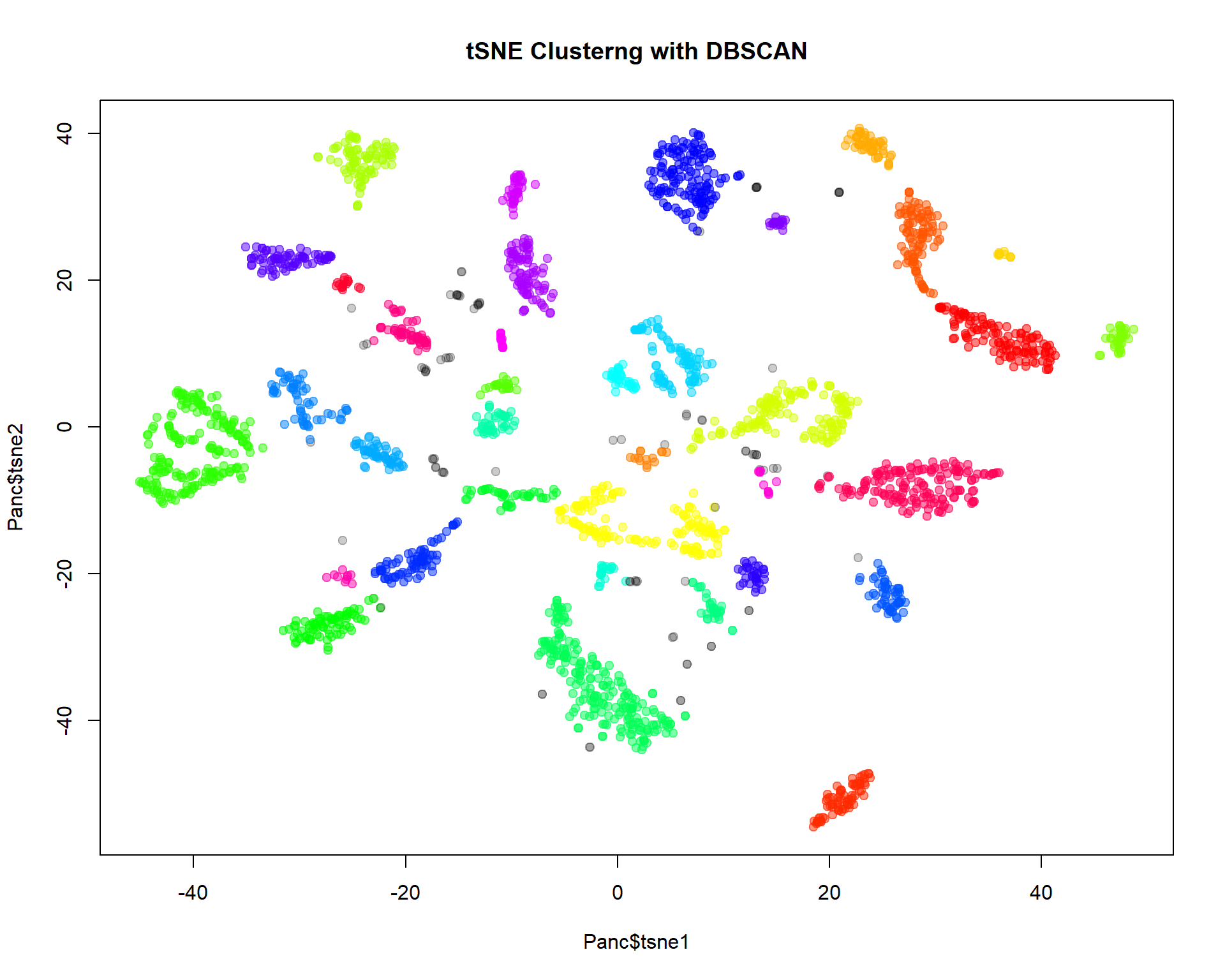

Exercises

Try kmeans and hclust for miRNA data (cluster both samples and the most variable genes). How many clusters would you use?

prcomp() kmeans(), dist(), hclust()

Investigate applicability of hclust and kmeans to t-SNE representation of Panc data.

dist(), hclust(), kmeans()

Prev Home

By Petr Nazarov