4. Methods for RNA-seq data
Petr V. Nazarov, LIH
2024-10-21
More detailed tutorials you could find on external resources, e.g.:
4.1. Analysis of RNA-seq data
For simplicity, let’s consider here how to run our custom warp-up function to analyse RNA-Seq data. If you are interested in using original Bioconductor functions - feel free to see in the code of LibDEA
Let’s consider the following libraries:
- DESeq2 is the one most often used (subjective), but it is also the slowest one (objective). It needs raw counts (negative binomial model of signal). It is developed by the group of Wolgang Huber (Heidelberg)
- edgeR . It needs raw counts (negative binomial model of signal). It is developed by the group of Gordon Smyth (Australia)
- limma . It can work with any form of expression
(use
voomto transform from counts to log-expression). It is as well developed by the group of Gordon Smyth (Australia)
## load data
Data = read.table("http://edu.modas.lu/data/txt/counts.txt",header=T,sep="\t",row.names = 1)
str(Data)
## 'data.frame': 60411 obs. of 18 variables:
## $ SN327: int 11404 95 5058 4015 4137 266 77088 98 29717 1285 ...
## $ SN328: int 4652 112 4899 7001 6626 1161 41068 118 13984 1908 ...
## $ SN349: int 12880 107 5948 6573 4753 523 67236 169 25633 1952 ...
## $ SN354: int 5252 149 6508 5730 4728 813 56781 250 10469 1830 ...
## $ SN405: int 7752 169 4596 5858 2926 221 62818 159 13303 1326 ...
## $ SN449: int 12215 161 4009 4811 3754 620 70614 67 16995 1281 ...
## $ SN450: int 10898 86 5288 5010 3051 1012 107658 142 20073 1592 ...
## $ SN667: int 9793 370 4371 4905 3563 118 78049 98 27813 2248 ...
## $ SN679: int 7039 340 3560 4215 2478 949 62394 120 6482 1036 ...
## $ ST327: int 1768 32 3346 6450 8849 46 27302 125 165479 1653 ...
## $ ST328: int 3944 7 5062 6055 5424 1483 24056 185 47563 2947 ...
## $ ST349: int 4703 54 5837 7117 7773 644 22856 178 94699 2573 ...
## $ ST354: int 6323 247 8614 5027 8724 83 8912 79 8426 3487 ...
## $ ST405: int 1496 16 2546 4677 6252 120 27303 143 70070 1364 ...
## $ ST449: int 5547 33 4912 6942 9630 693 15821 217 87792 2248 ...
## $ ST450: int 6467 131 5055 4591 7006 1053 33937 101 104311 2242 ...
## $ ST667: int 2136 43 4608 3955 4599 180 14647 154 41703 1185 ...
## $ ST679: int 2778 123 1938 1945 2587 909 13117 179 6037 1818 ...## load annotation
Anno = read.table("http://edu.modas.lu/data/txt/counts_anno.txt",header=T,sep="\t",row.names = 1, as.is=TRUE)
Anno = Anno[rownames(Data),] ## force the same order
str(Anno)## 'data.frame': 60411 obs. of 8 variables:
## $ gene_name : chr "TSPAN6" "TNMD" "DPM1" "SCYL3" ...
## $ gene_biotype: chr "protein_coding" "protein_coding" "protein_coding" "protein_coding" ...
## $ seqname : chr "X" "X" "20" "1" ...
## $ start : int 99884983 99839799 49551773 169822913 169631245 27939633 196621008 143816984 53363765 41040684 ...
## $ stop : int 99894942 99854882 49574900 169863148 169823221 27961576 196716634 143832548 53481684 41067715 ...
## $ strand : chr "-" "+" "-" "-" ...
## $ length : int 2968 1610 1207 3844 6354 3524 8144 2453 8463 3811 ...
## $ gc : num 0.441 0.425 0.398 0.445 0.423 ...This dataset contains 18 samples from 9 lung squamous cell carcinoma patients. Each tumor sample is paired with the normal. Below we will use 3 methods to exptract differentially expessed genes. Feel free to check LibDEA.r for more details.
edgeR - method developed by the same group as
limma. It assumes negative binomial distribution of the dataDESeq2 - method developed by W.Huber’s lab in Heidelberg
limma + voom - limma still can be used for counting data
source("http://r.modas.lu/LibDEA.r")## [1] "----------------------------------------------------------------"
## [1] "libDEA: Differential expression analysis"
## [1] "Needed:"
## [1] "limma" "edgeR" "DESeq2" "caTools" "compiler" "sva"
## [1] "Absent:"
## character(0)group = sub("[0-9]+","",colnames(Data))
## using DESeq2
Res1 = DEA.DESeq(Data, group=group, key0="SN", key1="ST")##
## DESeq,unpaired: 11920 DEG (FDR<0.05), 8913 DEG (FDR<0.01)## using edgeR
Res2 = DEA.edgeR(Data, group=group, key0="SN",key1="ST")##
## edgeR,unpaired: 8566 DEG (FDR<0.05), 5990 DEG (FDR<0.01)## using edgeR
Res3 = DEA.limma(Data, group=group, key0="SN",key1="ST",counted=TRUE)##
## Limma,unpaired: 9038,6004,3329,1767 DEG (FDR<0.05, 1e-2, 1e-3, 1e-4)The results are not the same. Let’s see:
## Venn diagram
library(gplots)

id1 = Res1[Res1$FDR<0.01 & abs(Res1$logFC)>1,"id"]
id2 = Res2[Res2$FDR<0.01 & abs(Res2$logFC)>1,"id"]
id3 = Res3[Res3$FDR<0.01 & abs(Res3$logFC)>1,"id"]

venn(list(DESeq = id1, edgeR=id2, limma = id3))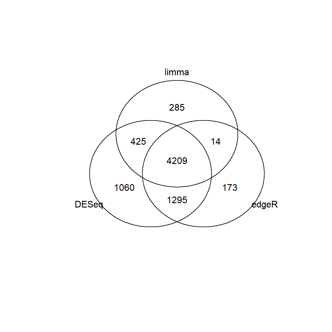
## alternative Venn
# source("http://r.modas.lu/Venn.r")
# v = Venn(list(DESeq = id1, edgeR=id2, limma = id3))
Exercise 4
To DO: Annotate data for task 4!
- Analyze dataset LUSC60 using one of the methods (DESeq2, edgeR or limma) and compare the gene lists to those found in LIH dataset counts. Sample annotation is quite straitforward: SN - normal, ST - tumour, but can also be found in samples.txt Hint: you will need to translate genes from Ensembl to gene symbols using anno
Alternatively: generate your own “AMD” file in Excel as described in session on Exploratory Data Analysis, section 1.2.1.
DEA.limma,DEA.DESeq,DEA.edgeRsub,venn
- Select the top 1000 of the significant genes either in LUSC20 or in counts, save gene names into a file and perform enrichment analysis using Enrichr tool of Icahn School of Medicine at Mount Sinai, NY, USA.
write
| Prev Home |
By Petr Nazarov
|