1. Basic statistics

1.1. Hypothesis testing and p-value

Here are few slides explaining the concept of hypothesis testing and p-value:

1.2. Parametric test for means (t-test)

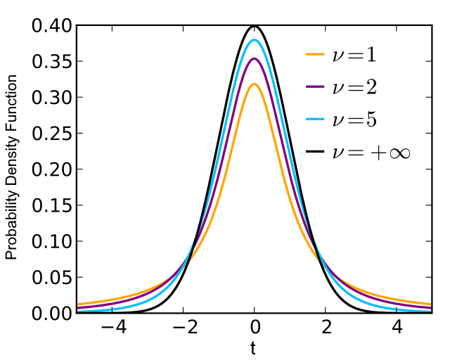
When we work with real data, we need to estimate variance based on experimental observation. This adds additional randomeness => sampling distribution (uncertainty) of mean follows Student (t) distribution.

Student distribution (Wikipedia)

Simple (unpaired) t-test

Let’s test, whether mean weight change differs for male & female mice. Animals in the groups are different, therefore we use unpaired t-test. Corresponding function is t.test()

## load data
Mice=read.table("http://edu.modas.lu/data/txt/mice.txt",header=T,sep="\t",as.is=FALSE)

xm = Mice$Weight.change[Mice$Sex=="m"]
xf = Mice$Weight.change[Mice$Sex=="f"]
t.test(xm,xf)

## 
##  Welch Two Sample t-test
## 
## data:  xm and xf
## t = 3.2067, df = 682.86, p-value = 0.001405
## alternative hypothesis: true difference in means is not equal to 0
## 95 percent confidence interval:
##  0.009873477 0.041059866
## sample estimates:
## mean of x mean of y 
##  1.119401  1.093934

## you can also compare to a constant
## check whether weight change is over 1:
t.test(xm, mu = 1, alternative = c("greater"))

## 
##  One Sample t-test
## 
## data:  xm
## t = 27.334, df = 393, p-value < 2.2e-16
## alternative hypothesis: true mean is greater than 1
## 95 percent confidence interval:
##  1.112199      Inf
## sample estimates:
## mean of x 
##  1.119401

Paired t-test

Example. The systolic blood pressures of n=12 women between the ages of 20 and 35 were measured before and after usage of a newly developed oral contraceptive.

BP=read.table("http://edu.modas.lu/data/txt/bloodpressure.txt",header=T,sep="\t")
str(BP)

## 'data.frame':    12 obs. of  3 variables:
##  $ Subject  : int  1 2 3 4 5 6 7 8 9 10 ...
##  $ BP.before: int  122 126 132 120 142 130 142 137 128 132 ...
##  $ BP.after : int  127 128 140 119 145 130 148 135 129 137 ...

## unpaired
t.test(BP$BP.before,BP$BP.after)

## 
##  Welch Two Sample t-test
## 
## data:  BP$BP.before and BP$BP.after
## t = -0.83189, df = 21.387, p-value = 0.4147
## alternative hypothesis: true difference in means is not equal to 0
## 95 percent confidence interval:
##  -9.034199  3.867532
## sample estimates:
## mean of x mean of y 
##  130.6667  133.2500

## paired
t.test(BP$BP.before,BP$BP.after,paired=T)

## 
##  Paired t-test
## 
## data:  BP$BP.before and BP$BP.after
## t = -2.8976, df = 11, p-value = 0.01451
## alternative hypothesis: true mean difference is not equal to 0
## 95 percent confidence interval:
##  -4.5455745 -0.6210921
## sample estimates:
## mean difference 
##       -2.583333

par(mfcol=c(1,2))
plot(BP$BP.before,BP$BP.after,pch=19,main="Blood pressure")
abline(a=0,b=1,lty=2,col=2)

plot(BP$BP.after-BP$BP.before,pch=19,main="Difference ")
abline(h=0,lty=2,col=2)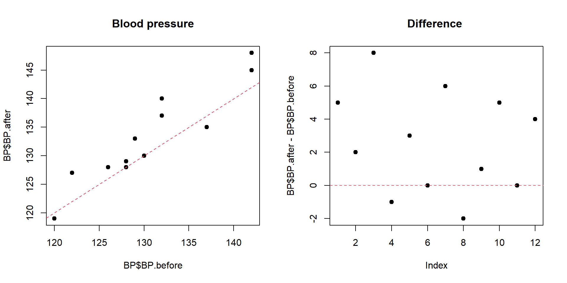

1.3. Non-parametric tests

The Mann–Whitney U test (a.k.a Mann–Whitney–Wilcoxon, Wilcoxon rank-sum, Wilcoxon–Mann–Whitney) is a nonparametric analogue of simple (unpaired) t-test
The Wilcoxon signed-rank test is a non-parametric analogue of a paired t-test

Both tests can be done in R with one command wilcox.test()

## unpaired
wilcox.test(BP$BP.before,BP$BP.after)

## 
##  Wilcoxon rank sum test with continuity correction
## 
## data:  BP$BP.before and BP$BP.after
## W = 59.5, p-value = 0.487
## alternative hypothesis: true location shift is not equal to 0

## paired
wilcox.test(BP$BP.before,BP$BP.after,paired=TRUE)

## 
##  Wilcoxon signed rank test with continuity correction
## 
## data:  BP$BP.before and BP$BP.after
## V = 5, p-value = 0.02465
## alternative hypothesis: true location shift is not equal to 0

1.4. Testing variance

The ratio of sample variances for 2 samples from the same population follows F-distribution (a.k.a. Fisher–Snedecor distribution).

F-distribution (Wikipedia)

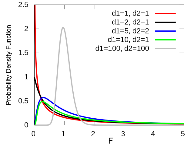
You can compare variances of 2 samples using var.test()

Example. A school is selecting a company to provide school bus to its pupils. They would like to choose the most punctual one. The times between bus arrival of two companies were measured and stored in schoolbus dataset. Please test whether the difference is significant with $\alpha = 0.1$.

Bus=read.table("http://edu.modas.lu/data/txt/schoolbus.txt",header=T,sep="\t")
str(Bus)

## 'data.frame':    26 obs. of  2 variables:
##  $ Milbank  : num  35.9 29.9 31.2 16.2 19 15.9 18.8 22.2 19.9 16.4 ...
##  $ Gulf.Park: num  21.6 20.5 23.3 18.8 17.2 7.7 18.6 18.7 20.4 22.4 ...

# see variances
apply(Bus,2,var,na.rm=TRUE)

##   Milbank Gulf.Park 
##  48.02062  19.99996

# test whether they could be the same
var.test(Bus[,1], Bus[,2])

## 
##  F test to compare two variances
## 
## data:  Bus[, 1] and Bus[, 2]
## F = 2.401, num df = 25, denom df = 15, p-value = 0.08105
## alternative hypothesis: true ratio of variances is not equal to 1
## 95 percent confidence interval:
##  0.8927789 5.7887880
## sample estimates:
## ratio of variances 
##           2.401036

Exercise 1

Compare Ending.weight for male and female mice of 129S1/SvImJ strain

t.test(), Mice$Ending.weight, Mice$Strain == "129S1/SvImJ" & Mice$Sex=="m"

Compare Bleeding.time between CAST/EiJ and NON/ShiLtJ (case sensitive!) using parametric and non-parametric tests.

t.test(), wilcoxon.test()

Home Next

By Petr Nazarov