3. LIMMA - Linear Models for Microarray Data
Petr V. Nazarov, LIH
2024-10-21
3.1. Installation of the required libraries
In the native R, the vast majority of the libraries (or packages) can
be simply installed by install.libraries("library_name").
However, some advanced R/Bioconductor packages may need advanced
handling of the dependencies. Thus, we would recommend using
BiocManager::install() function:
if (!requireNamespace("BiocManager", quietly = TRUE))
    install.packages("BiocManager")

BiocManager::install("limma")
BiocManager::install("edgeR")
BiocManager::install("DESeq2")
DESeq2 (developed in EMBL, Heidelberg) is very powerful but the most demanding package in terms of dependencies :)… Please try to install all 3 packages.
3.2. Analysis of microarrays
3.2.1 General information and data loading
Here we will consider only modern one-color arrays. However the methods were developed and are applicable for two-color arrays.
If you work with Affymetrix (now ThermoFisher) one-colour arrays - be prepared that some preliminary step should be performed before you can really touch the data. Binary CEL files should be processed by one of the tools, probe intensity normalized and summarized into probesets (old arrays and arrays targeted at splicing) or transcript clusters. The later is (to some extent) a synonym for “genes”. Some tools that can help are listed below:
Trancriptome Analysis Console (TAC) - free and quite advanced tool. Allows import Affymetrix and Thermofisher (Clariom) arrays, RMA normalizations with GC correction, data visualization, statistical analysis and functional annotation. (strongly recommended for Affy/Thermo arrays)
Affymetrix Power Tools (APT) - free & flexible command line tools for older versions of Affymetrix arrays.
oligo package of R/Bioconductor - free tool for R geeks :). For example of application - see Exercise 6.1 of AdvBiostat course.
If you would like to check the results of TAC, please see these files:
HTA.txt contains expression measure by HTA 2.0 arrays
HTA_anno.txt - file with annotation.
Sample annotation is in samples.txt
Let’s load mRNA dataset from IFNg experiment
## importing readAMD script from Internet
source("http://r.modas.lu/readAMD.r")

## load mRNA data from IFNg experiment:
mRNA = readAMD("http://edu.modas.lu/data/txt/mrna_ifng.amd.txt",
               stringsAsFactors = TRUE,
               index.column="GeneSymbol",
               sum.func="mean")
3.2.2 limma - LInear Models for MicroArrays
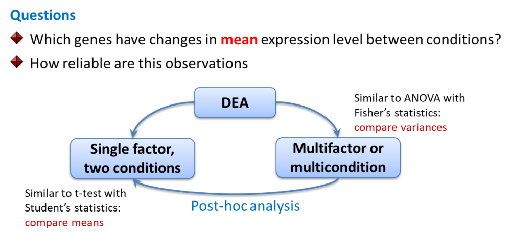
Limma works similar to ANOVA with somewhat improved post-hoc analysis and p-value calculation (empirical Bayes statistics). Let’s first see how to do simple analysis and then consider a warp-up function.
library(limma)
library(pheatmap)

## now create design matrix (a lot of "FUN" !)
design = model.matrix(~ -1 + mRNA$meta$time)
colnames(design)=sub(".+time","",colnames(design))
design
## T00 T03 T12 T24 T48 T72 T72J
## 1 1 0 0 0 0 0 0
## 2 1 0 0 0 0 0 0
## 3 0 1 0 0 0 0 0
## 4 0 1 0 0 0 0 0
## 5 0 0 1 0 0 0 0
## 6 0 0 1 0 0 0 0
## 7 0 0 0 1 0 0 0
## 8 0 0 0 1 0 0 0
## 9 0 0 0 1 0 0 0
## 10 0 0 0 0 1 0 0
## 11 0 0 0 0 1 0 0
## 12 0 0 0 0 1 0 0
## 13 0 0 0 0 0 1 0
## 14 0 0 0 0 0 1 0
## 15 0 0 0 0 0 1 0
## 16 0 0 0 0 0 0 1
## 17 0 0 0 0 0 0 1
## attr(,"assign")
## [1] 1 1 1 1 1 1 1
## attr(,"contrasts")
## attr(,"contrasts")$`mRNA$meta$time`
## [1] "contr.treatment"## first fit: linear model
fit = lmFit(mRNA$X,design=design)
colnames(design)## [1] "T00" "T03" "T12" "T24" "T48" "T72" "T72J"## define contrast (post-hoc of ANOVA)
contrast.matrix = makeContrasts(T03-T00,T12-T00,T24-T00,T48-T00,T72-T00,T72J-T00, levels=design)
contrast.matrix## Contrasts
## Levels T03 - T00 T12 - T00 T24 - T00 T48 - T00 T72 - T00 T72J - T00
## T00 -1 -1 -1 -1 -1 -1
## T03 1 0 0 0 0 0
## T12 0 1 0 0 0 0
## T24 0 0 1 0 0 0
## T48 0 0 0 1 0 0
## T72 0 0 0 0 1 0
## T72J 0 0 0 0 0 1## second fit: contrasts - like post-hoc in ANOVA
fit2 = contrasts.fit(fit,contrast.matrix)
EB = eBayes(fit2)
## get table of top 100 significant genes by F-statistics (most variable)
Top100 = topTable(EB,coef=NULL,number=100,adjust="BH", genelist = mRNA$anno$GeneSymbol)
str(Top100)## 'data.frame': 100 obs. of 11 variables:
## $ ProbeID : chr "C1S" "IDO1" "IGFBP5" "C9orf150" ...
## $ T03...T00 : num 0.78 5.242 -0.112 0.021 1.754 ...
## $ T12...T00 : num 2.8 7.621 -1.494 0.752 5.454 ...
## $ T24...T00 : num 4.11 6.84 -2.23 4.25 6.12 ...
## $ T48...T00 : num 4.7 5.2 -5.99 4.43 4.78 ...
## $ T72...T00 : num 4.51 3.83 -6.53 4.16 3.64 ...
## $ T72J...T00: num 0.813 1.1399 -1.7693 0.3305 0.0716 ...
## $ AveExpr : num 7.93 8.96 8.68 8.47 8.3 ...
## $ F : num 1809 1695 1508 1410 1235 ...
## $ P.Value : num 1.98e-21 3.32e-21 8.29e-21 1.41e-20 3.97e-20 ...
## $ adj.P.Val : num 3.34e-17 3.34e-17 5.57e-17 7.09e-17 1.53e-16 ...## visualize top 100 by F-stat
genes = Top100[,1]
pheatmap(mRNA$X[genes,],cluster_col=FALSE,fontsize_row=5,fontsize_col=10,cellwidth=15,scale="row",main="Top 100 variable genes (F-stat)")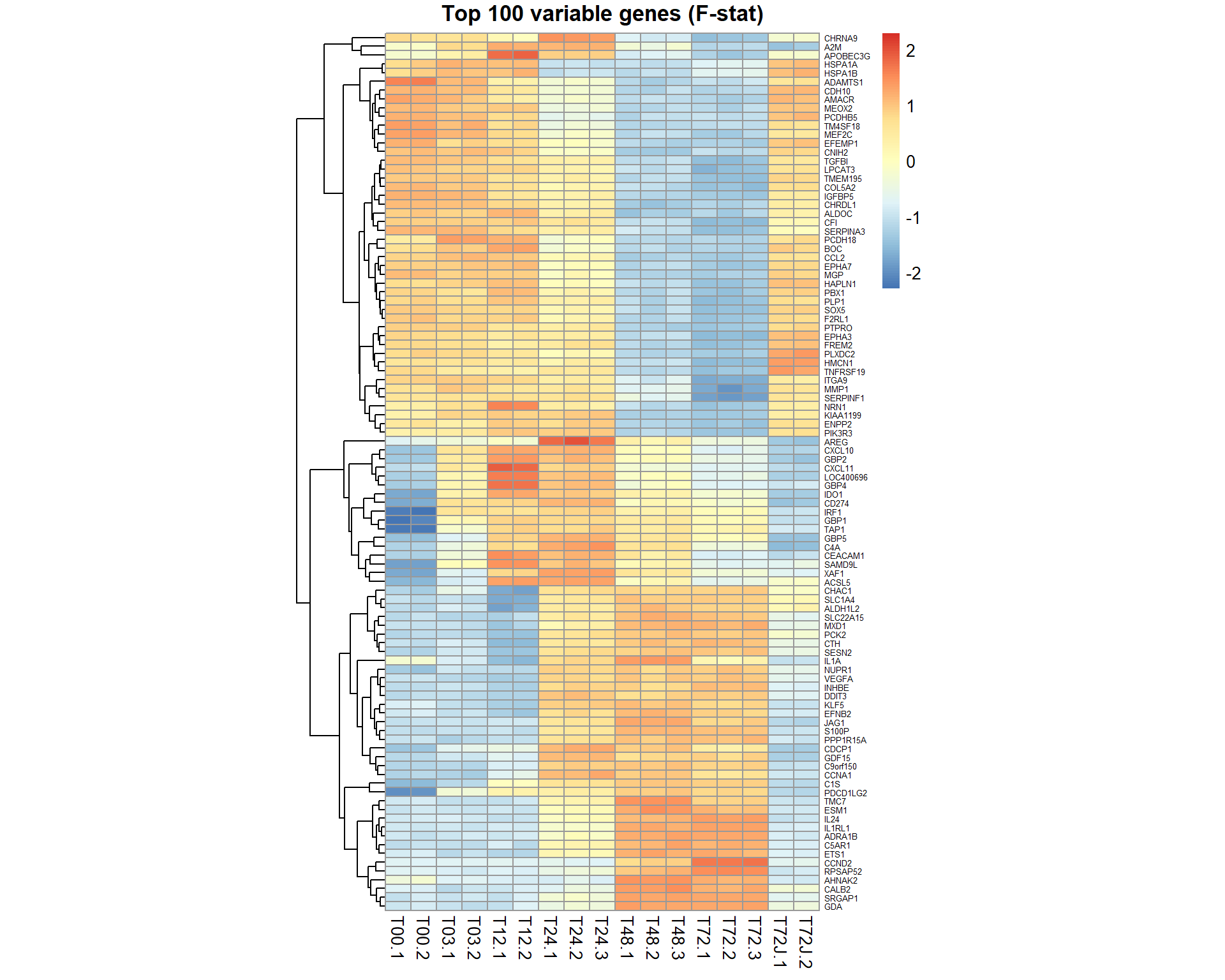
## get table of top 100 significant genes for the contrast "coef"
Top100 = topTable(EB,coef="T24 - T00",number=100,adjust="BH", genelist = mRNA$anno$GeneSymbol)
str(Top100)
## 'data.frame': 100 obs. of 7 variables:
## $ ID : chr "IDO1" "IRF1" "C1S" "GBP5" ...
## $ logFC : num 6.84 5.18 4.11 6.12 4.57 ...
## $ AveExpr : num 8.96 10.16 7.93 8.3 11.53 ...
## $ t : num 74.5 64.7 62.4 61.8 59.4 ...
## $ P.Value : num 1.76e-21 1.59e-20 2.79e-20 3.25e-20 6.07e-20 ...
## $ adj.P.Val: num 3.54e-17 1.60e-16 1.64e-16 1.64e-16 2.45e-16 ...
## $ B : num 37.2 35.7 35.3 35.2 34.7 ...## visualize top 100 by moderated t-test
genes = Top100[,1]
samples = grep("T00|T24",mRNA$meta$time)
pheatmap(mRNA$X[genes,samples],cluster_col=FALSE,fontsize_row=5,fontsize_col=10,cellwidth=15,scale="row", main="Top 100 genes: T24 - T00 (t-stat)")
3.2.3 DEA.limma - warp-up of the standard limma
analysis
Now we do the same with a warp-up function
DEA.limma()
source("http://r.modas.lu/LibDEA.r")## [1] "----------------------------------------------------------------"
## [1] "libDEA: Differential expression analysis"
## [1] "Needed:"
## [1] "limma" "edgeR" "DESeq2" "caTools" "compiler" "sva"
## [1] "Absent:"
## character(0)## most variable (by F-stat)
ResF = DEA.limma(data = mRNA$X,
group = mRNA$meta$time)## [1] "T03-T00" "T12-T00" "T12-T03" "T24-T00" "T24-T03" "T24-T12"
## [7] "T48-T00" "T48-T03" "T48-T12" "T48-T24" "T72-T00" "T72-T03"
## [13] "T72-T12" "T72-T24" "T72-T48" "T72J-T00" "T72J-T03" "T72J-T12"
## [19] "T72J-T24" "T72J-T48" "T72J-T72"
##
## Limma,unpaired: 11468,9604,7444,5630 DEG (FDR<0.05, 1e-2, 1e-3, 1e-4)str(ResF)## 'data.frame': 20141 obs. of 26 variables:
## $ id : chr "" "A1BG" "A1CF" "A2BP1" ...
## $ T03.T00 : num -0.0237 0.0997 0.0557 -0.033 -0.0733 ...
## $ T12.T00 : num 0.00463 0.21845 0.11754 -0.06136 -0.27599 ...
## $ T12.T03 : num 0.0283 0.1188 0.0618 -0.0284 -0.2027 ...
## $ T24.T00 : num -0.009247 -0.000912 0.13822 0.055437 0.140712 ...
## $ T24.T03 : num 0.0144 -0.1006 0.0825 0.0884 0.2141 ...
## $ T24.T12 : num -0.0139 -0.2194 0.0207 0.1168 0.4167 ...
## $ T48.T00 : num 0.0123 0.1058 0.185 0.0644 0.2249 ...
## $ T48.T03 : num 0.03601 0.00611 0.12927 0.0973 0.29828 ...
## $ T48.T12 : num 0.00772 -0.11264 0.06747 0.12571 0.50093 ...
## $ T48.T24 : num 0.02159 0.10672 0.04679 0.00891 0.08422 ...
## $ T72.T00 : num -0.0361 0.081 0.0831 0.0756 0.3512 ...
## $ T72.T03 : num -0.0125 -0.0187 0.0273 0.1086 0.4245 ...
## $ T72.T12 : num -0.0408 -0.1374 -0.0345 0.137 0.6272 ...
## $ T72.T24 : num -0.0269 0.0819 -0.0551 0.0202 0.2105 ...
## $ T72.T48 : num -0.0485 -0.0248 -0.1019 0.0113 0.1262 ...
## $ T72J.T00: num -0.0337 0.0947 0.0557 -0.0732 -0.0356 ...
## $ T72J.T03: num -0.01 -0.00504 -0.00004 -0.04028 0.03771 ...
## $ T72J.T12: num -0.0383 -0.1238 -0.0618 -0.0119 0.2404 ...
## $ T72J.T24: num -0.0244 0.0956 -0.0825 -0.1287 -0.1763 ...
## $ T72J.T48: num -0.046 -0.0112 -0.1293 -0.1376 -0.2606 ...
## $ T72J.T72: num 0.00248 0.01365 -0.02738 -0.14884 -0.38682 ...
## $ AveExpr : num 6.6 6.25 5.1 4.64 5.92 ...
## $ F : num 0.206 1.115 0.752 1.105 12.274 ...
## $ PValue : num 9.70e-01 3.97e-01 6.17e-01 4.02e-01 3.62e-05 ...
## $ FDR : num 0.974899 0.48257 0.683201 0.487241 0.000126 ...genes = order(ResF$FDR)[1:100] ## select top 100
genes = ResF$id[ResF$FDR < 1e-6] ## select all significant with FDR<0.000001
pheatmap(mRNA$X[genes,],cluster_col=FALSE,fontsize_row=2,fontsize_col=10,cellwidth=15,scale="row",main="Top 100 variable genes (F-stat)")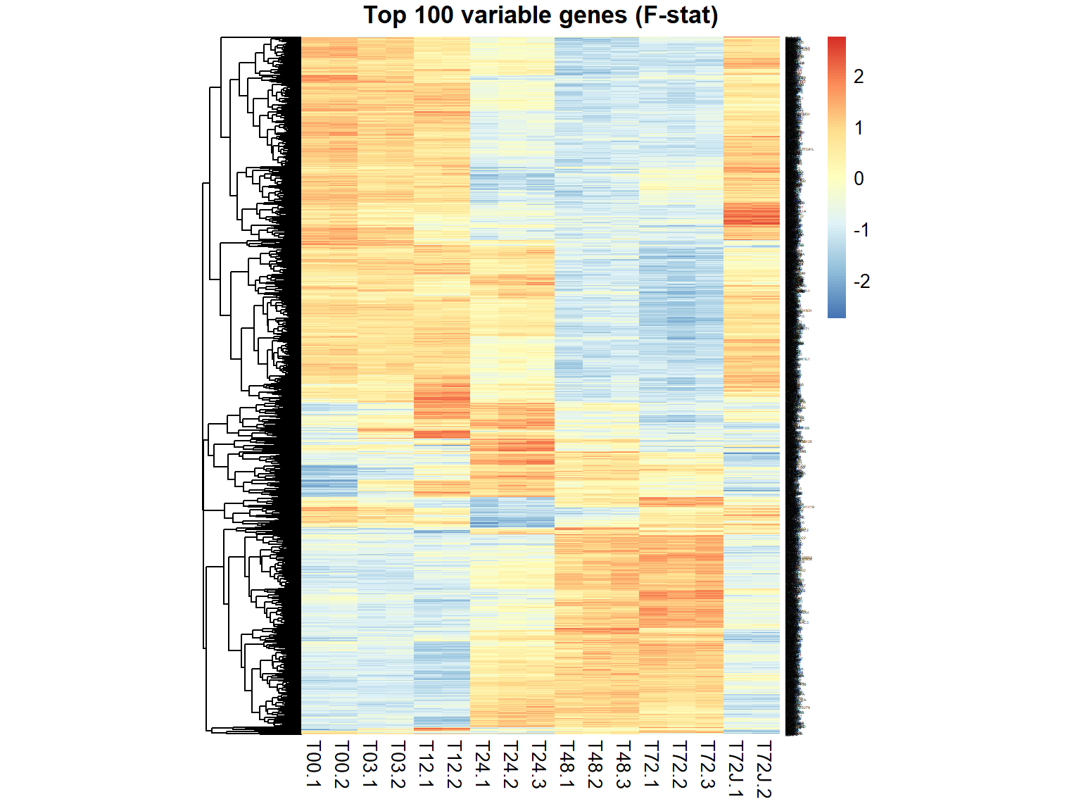
## T24 - T00
Res24 = DEA.limma(data = mRNA$X,
                group = mRNA$meta$time,
                key0="T00",
                key1="T24")
##
## Limma,unpaired: 5895,3980,2146,1023 DEG (FDR<0.05, 1e-2, 1e-3, 1e-4)## now let's plot volcano
plotVolcano(Res24,thr.fdr=0.01,thr.lfc=1)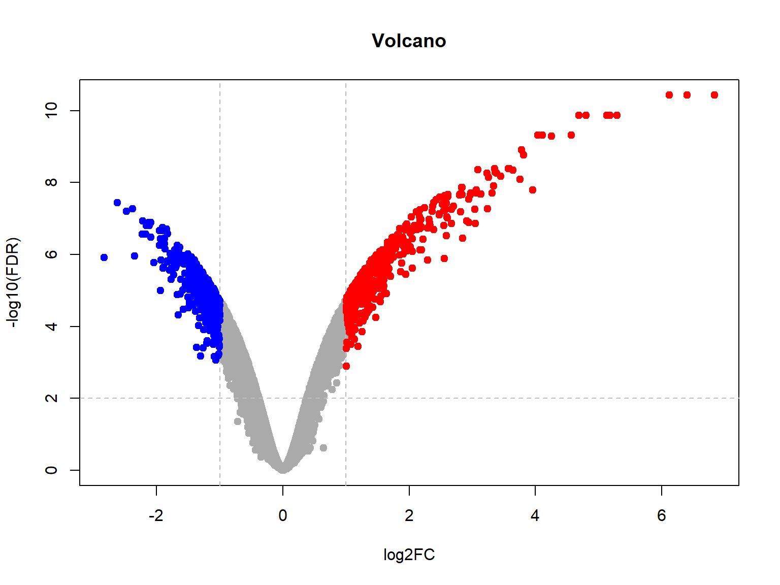
One controversial point is, whether all data should be used for the analysis, or only the one mentioned in the contrast? Often for safety reasons people would like to limit data to the current conditions in the contrast. It decrease sensitivity, but make analysis more robust to changes in other samples.
Finally, let’s save significant data, i.e. with FDR<0.01 to the disk.
str(ResF)
write.table(ResF[ResF$FDR<0.0001,], "DEA_F.txt",col.names=NA,sep="\t",quote=FALSE)

str(Res24)
write.table(Res24[Res24$FDR<0.001 & abs(Res24$logFC)>1,],
            file = "DEA_T24-T00.txt",col.names=NA,sep="\t",quote=FALSE)
3.3. Functional annotation
There are tools for functional annotations in R. But for the sake of time, let’s use one of the public tools: Enrichr
Save you significant genes to a file
Put them into the Enrichr tool
write(Res24$id[Res24$FDR<0.001 & abs(Res24$logFC)>1],
            file = "genes_T24-T00.txt")
Exercise 3
- For mRNA data mRNA, calculate the number of significant genes (FDR<0.01) for each time point vs. T00. Visualize as barplot
DEA.limma(),sum(Res$FDR<0.01),barplot()
- Analyze dataset miRNA using either native limma or
DEA.limma()warpup. Calculate the number of significant miRNA between untreated samples and each time point.
DEA.limma()Whether mRNA or miRNA respond faster to IFNg stimulation?
| Prev Home Next |
By Petr Nazarov
|