2. Multiple testing. ANOVA
Petr V. Nazarov, LIH
2024-10-21
Here are few slides explaining the problems of multiple hypothesis testing and the concept of ANOVA: analysis of variance.
Multiple testing, ANOVA Partek’s ANOVA
2.1. Multiple hypothesis testing
Let’s run a small test described in the lecture: generate a random dataset with 1000 “genes” for 6 “samples”. 3 samples we denote as “A”, 3 - as “B”
library(pheatmap)

ng = 1000  ## n genes
nr = 3     ## n replicates

## random matrix
X = matrix(rnorm(ng*nr*2),nrow=ng, ncol=nr*2)
rownames(X) = paste0("gene",1:ng)
colnames(X) = c(paste0("A",1:nr),paste0("B",1:nr))
pheatmap(X,fontsize_row = 1,cellwidth=20,main="Random expression matrix",scale="row")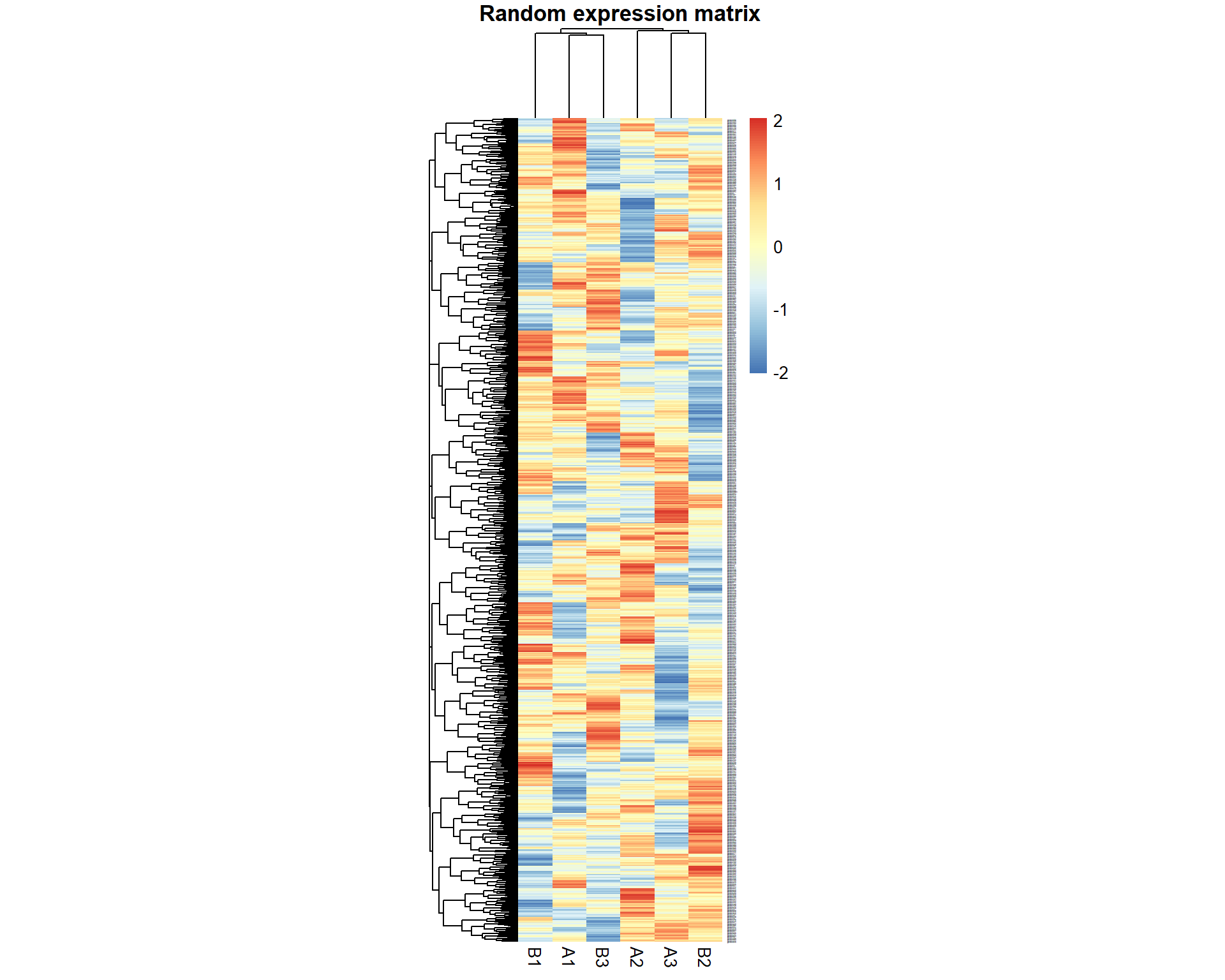
## calculate p-values
pv = double(ng)
names(pv) = rownames(X)
for (i in 1:ng){
  pv[i] = t.test(X[i,1:nr],X[i,(nr+1):(2*nr)])$p.value
}
pheatmap(X[pv<0.05,],cellwidth=20,main="Significant genes by p-value",scale="row")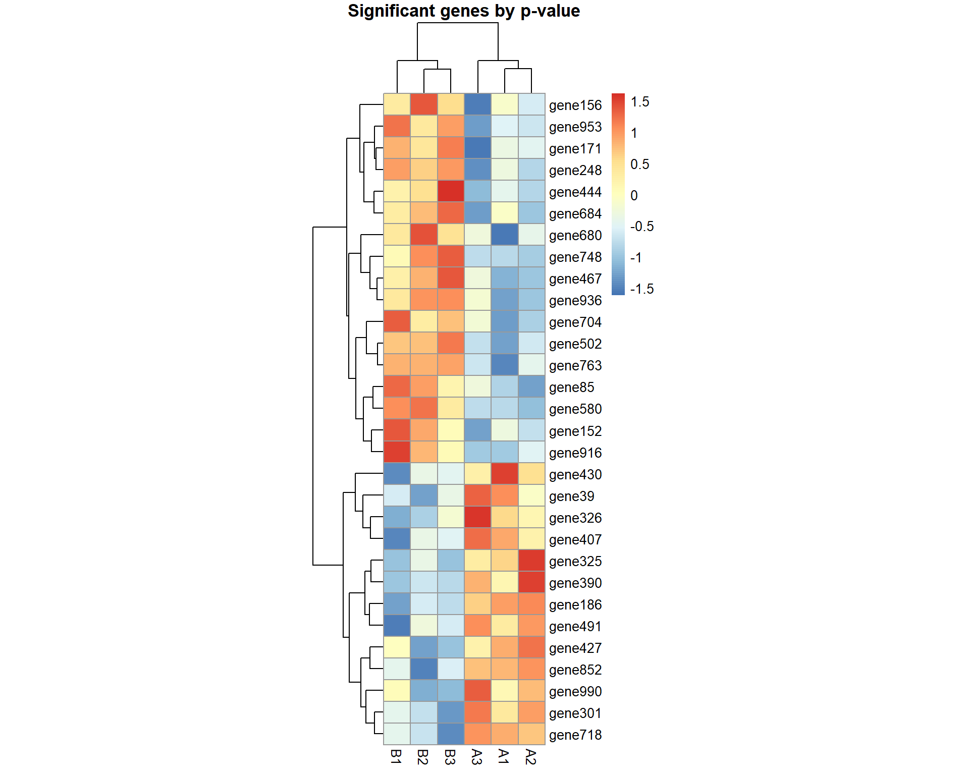
## Significant genes by p-value:
print(names(pv)[pv<0.05])
## [1] "gene19" "gene59" "gene63" "gene105" "gene119" "gene179" "gene247"
## [8] "gene377" "gene422" "gene467" "gene473" "gene504" "gene521" "gene560"
## [15] "gene573" "gene623" "gene640" "gene642" "gene651" "gene684" "gene740"
## [22] "gene815" "gene851" "gene857" "gene875" "gene900" "gene914" "gene919"
## [29] "gene972" "gene983"## Correction for multiple testing using Benjamini-Hochberg's FDR and Holm's FWER
fdr = p.adjust(pv,"fdr")
fwer = p.adjust(pv,"holm")
## Significant genes by FDR:
print(names(fdr)[fdr<0.05])## character(0)data.frame(PV=pv[pv<0.05],FDR=fdr[pv<0.05],FWER=fwer[pv<0.05])## PV FDR FWER
## gene19 0.015734626 0.9850286 1
## gene59 0.045981327 0.9850286 1
## gene63 0.037207845 0.9850286 1
## gene105 0.006194036 0.9850286 1
## gene119 0.021669356 0.9850286 1
## gene179 0.021919625 0.9850286 1
## gene247 0.037145409 0.9850286 1
## gene377 0.035298244 0.9850286 1
## gene422 0.031102847 0.9850286 1
## gene467 0.029243613 0.9850286 1
## gene473 0.023295851 0.9850286 1
## gene504 0.014021406 0.9850286 1
## gene521 0.020510770 0.9850286 1
## gene560 0.019365928 0.9850286 1
## gene573 0.041391758 0.9850286 1
## gene623 0.015333000 0.9850286 1
## gene640 0.042572849 0.9850286 1
## gene642 0.021568229 0.9850286 1
## gene651 0.037724627 0.9850286 1
## gene684 0.027078113 0.9850286 1
## gene740 0.012795300 0.9850286 1
## gene815 0.043454476 0.9850286 1
## gene851 0.041539004 0.9850286 1
## gene857 0.018237053 0.9850286 1
## gene875 0.047861100 0.9850286 1
## gene900 0.025393720 0.9850286 1
## gene914 0.012395987 0.9850286 1
## gene919 0.005146961 0.9850286 1
## gene972 0.042162812 0.9850286 1
## gene983 0.012836655 0.9850286 12.2. Analysis of Variance (ANOVA)
## load data
Dep = read.table("http://edu.modas.lu/data/txt/depression2.txt",header=T,sep="\t",as.is=FALSE)
str(Dep)
## 'data.frame': 120 obs. of 3 variables:
## $ Location : Factor w/ 3 levels "Florida","New York",..: 1 1 1 1 1 1 1 1 1 1 ...
## $ Health : Factor w/ 2 levels "bad","good": 2 2 2 2 2 2 2 2 2 2 ...
## $ Depression: int 3 7 7 3 8 8 8 5 5 2 ...2.2.1. One-way (one-factor) ANOVA
We start with one-way ANOVA. Let’s consider only healthy respondents
in Dep dataset. ANOVA is performed in R:
aov(formula, data)
formula- “Values ~ Factor1”, where “Values”, “Factor1” should be replaced by the actual column names in the data framedata
ANOVA tells whether a factor is significant, but tells nothing with
treatments (factor levels) are different! Use TukeyHSD() to
perform post-hoc analysis and get corrected p-values for the
contrasts.
DepGH = Dep[Dep$Health == "good",]

## build 1-factor ANOVA model
res1 = aov(Depression ~  Location, DepGH)
summary(res1)
## Df Sum Sq Mean Sq F value Pr(>F)
## Location 2 78.5 39.27 6.773 0.0023 **
## Residuals 57 330.4 5.80
## ---
## Signif. codes: 0 '***' 0.001 '**' 0.01 '*' 0.05 '.' 0.1 ' ' 1TukeyHSD(res1)## Tukey multiple comparisons of means
## 95% family-wise confidence level
##
## Fit: aov(formula = Depression ~ Location, data = DepGH)
##
## $Location
## diff lwr upr p adj
## New York-Florida 2.8 0.9677423 4.6322577 0.0014973
## North Carolina-Florida 1.5 -0.3322577 3.3322577 0.1289579
## North Carolina-New York -1.3 -3.1322577 0.5322577 0.21126122.2.2. Two-way (two-factor) ANOVA
For two-way ANOVA the call is similar
aov(formula, data). Please note that factor columns in the
data frame data should be of class "factor"
(newer R version accepts "character"). If factors are
"numeric", aov will build regression instead.
formula- “Values ~ Factor1 + Factor2 + Factor1*Factor2”, where “Values”, “Factor1” and “Factor2” should be replaced by the actual column names in the data framedataInteraction “Factor1*Factor2” can be estimated in case, if you table contains replicates (values measured for the same conditions)
If needed, ANOVA can be followed by TukeyHSD().
## build 2-factor ANOVA model (with interaction)
res2 = aov(Depression ~  Location + Health + Location*Health, Dep)
summary(res2)
## Df Sum Sq Mean Sq F value Pr(>F)
## Location 2 73.8 36.9 4.290 0.016 *
## Health 1 1748.0 1748.0 203.094 <2e-16 ***
## Location:Health 2 26.1 13.1 1.517 0.224
## Residuals 114 981.2 8.6
## ---
## Signif. codes: 0 '***' 0.001 '**' 0.01 '*' 0.05 '.' 0.1 ' ' 1TukeyHSD(res2)## Tukey multiple comparisons of means
## 95% family-wise confidence level
##
## Fit: aov(formula = Depression ~ Location + Health + Location * Health, data = Dep)
##
## $Location
## diff lwr upr p adj
## New York-Florida 1.850 0.2921599 3.4078401 0.0155179
## North Carolina-Florida 0.475 -1.0828401 2.0328401 0.7497611
## North Carolina-New York -1.375 -2.9328401 0.1828401 0.0951631
##
## $Health
## diff lwr upr p adj
## good-bad -7.633333 -8.694414 -6.572252 0
##
## $`Location:Health`
## diff lwr upr p adj
## New York:bad-Florida:bad 0.90 -1.7893115 3.589311 0.9264595
## North Carolina:bad-Florida:bad -0.55 -3.2393115 2.139311 0.9913348
## Florida:good-Florida:bad -8.95 -11.6393115 -6.260689 0.0000000
## New York:good-Florida:bad -6.15 -8.8393115 -3.460689 0.0000000
## North Carolina:good-Florida:bad -7.45 -10.1393115 -4.760689 0.0000000
## North Carolina:bad-New York:bad -1.45 -4.1393115 1.239311 0.6244461
## Florida:good-New York:bad -9.85 -12.5393115 -7.160689 0.0000000
## New York:good-New York:bad -7.05 -9.7393115 -4.360689 0.0000000
## North Carolina:good-New York:bad -8.35 -11.0393115 -5.660689 0.0000000
## Florida:good-North Carolina:bad -8.40 -11.0893115 -5.710689 0.0000000
## New York:good-North Carolina:bad -5.60 -8.2893115 -2.910689 0.0000003
## North Carolina:good-North Carolina:bad -6.90 -9.5893115 -4.210689 0.0000000
## New York:good-Florida:good 2.80 0.1106885 5.489311 0.0361494
## North Carolina:good-Florida:good 1.50 -1.1893115 4.189311 0.5892328
## North Carolina:good-New York:good -1.30 -3.9893115 1.389311 0.7262066TukeyHSD() output may be quite long. If you wish saving
it to a text file for later analysis - use sink()
function
## start writing logs to the file
sink("tukey.txt")
## print output
TukeyHSD(res2)
## close the file and write it to the current folder
sink()
Exercise 2
- Dataset teeth2 contains the result of an experiment, conducted to measure the effect of various doses of vitamin C on the tooth growth (model animal – Guinea pigs). Vitamin C and orange juice were given to animals in different quantities. Using 2-way ANOVA study the effects of vitamin-C and orange juice. Transform Dose to a factor.
factor(),aov(),summary()
- Each of six garter snakes (Thamnophis radix) was observed during the presentation of petri dishes containing solutions of different chemical stimuli. The number of tongue flicks during a 5-minute interval of exposure was recorded. The three petri dishes were presented to each snake in random order. See data in “snakes” table. Does solution affect tongue flicks? Should we correct the results for effect of difference b/w snakes (1- or 2-factor ANOVA)? Perform post hoc analysis for the significant factor. Use snakes dataset. It should be transformed before being used - see
meltofreshape2package.
str(),melt(Data,id=c("Snake")),aov,summary
| Prev Home Next |
By Petr Nazarov
|