Lecture 3. Linear models
Petr V. Nazarov, LIH
2024-03-04
| Materials: Presentation Tasks |
3.1. INFERENCE ABOUT VARIANCE
3.1.1 Interval estimation
Sampling distribution of \(\frac{(n-1)s^2}{\sigma^2}\) Whenever a simple random sample of size n is selected from a normal population, the sampling distribution of \(\frac{(n-1)s^2}{\sigma^2}\) has a chi-square distribution (\(\chi^2\)) with \(n-1\) degrees of freedom.
Example: Suppose sample of n = 36 coffee cans is selected and m = 2.92 and s = 0.18 lbm is observed. Provide 95% confidence interval for the standard deviation
We can use formula:
\[\frac{(n-1)s^2}{\chi_{1-\alpha/2}^2} \le \sigma^2 \le \frac{(n-1)s^2}{\chi_{\alpha/2}^2}\]
n = 36    # sample size
s = 0.18  # observed standard deviation (sqrt of variance)
a = 0.05  # alpha

## lower limit of variance
s2min = (n-1)*s^2/qchisq(1-a/2, n-1)
## upper limit of variance
s2max = (n-1)*s^2/qchisq(a/2, n-1)

cat(sprintf("C.I.(%g%%) of the observed st.dev = %g lbm is (%.3f, %.3f)",
    (1-a)*100,s,sqrt(s2min),sqrt(s2max)))
## C.I.(95%) of the observed st.dev = 0.18 lbm is (0.146, 0.235)3.1.2 Hypotheses about variances
Sampling distribution of \(s_1^2/s_2^2\) when \(\sigma_1^2/\sigma_2^2\) Whenever a independent simple random samples of size \(n_1\) and \(n_2\) are selected from two normal populations with equal variances, the sampling of \(s_1^2/s_2^2\) has F-distribution with \(n_1-1\) degree of freedom for numerator and \(n_2-1\) for denominator.
In R we will simply use var.test().
Example: Compare variances of time between buses for 2 bus companies: Milbank and Gulf Park. Use \(\alpha = 0.1\).
Bus = read.table("http://edu.modas.lu/data/txt/schoolbus.txt",header=TRUE,sep="\t")
str(Bus)
## 'data.frame': 26 obs. of 2 variables:
## $ Milbank : num 35.9 29.9 31.2 16.2 19 15.9 18.8 22.2 19.9 16.4 ...
## $ Gulf.Park: num 21.6 20.5 23.3 18.8 17.2 7.7 18.6 18.7 20.4 22.4 ...var.test(Bus$Milbank,Bus$Gulf.Park)##
## F test to compare two variances
##
## data: Bus$Milbank and Bus$Gulf.Park
## F = 2.401, num df = 25, denom df = 15, p-value = 0.08105
## alternative hypothesis: true ratio of variances is not equal to 1
## 95 percent confidence interval:
## 0.8927789 5.7887880
## sample estimates:
## ratio of variances
## 2.4010363.2. GOODNESS OF FIT
Here we will discuss how to test whether distribution fit to the observations (or vice versa).
3.2.1. Testing models for multinomial experiment
Multinomial population - a population in which each element is assigned to one and only one of several categories. The multinomial distribution extends the binomial distribution from two to three or more outcomes.
Goodness of fit test - a statistical test conducted to determine whether to reject a hypothesized probability distribution for a population.
Model - our assumption concerning the distribution, which we would like to test. Observed frequency - frequency distribution for experimentally observed data \(f_i\). Expected frequency - frequency distribution, which we would expect from our model, \(e_i\)
Test statistics is \(\chi^2\) with \(k-1\) degree of freedom:
\[\chi_{k-1}^2 = \sum_{i=1}^{k} \frac{(f_i-e_i)^2}{e_i^2}\] NOTE: at least 5 observations are expected in each category! => \(e_i \ge 5\)
Example: The new treatment for a disease is tested on 200 patients. The outcomes are classified as:
- A – patient is completely treated
- B – disease transforms into a chronic form
- C – treatment is unsuccessful
In parallel the 100 patients treated with standard methods are observed

# input data
Tab = cbind(c(94,42,64),c(38,28,34))
colnames(Tab) = c("exp","ctrl")
rownames(Tab) = c("A","B","C")
print(Tab)
## exp ctrl
## A 94 38
## B 42 28
## C 64 34# control defines Model
mod=Tab[,2]/sum(Tab[,2])
# test Model for 'exp'
chisq.test(Tab[,1],p=mod)##
## Chi-squared test for given probabilities
##
## data: Tab[, 1]
## X-squared = 7.9985, df = 2, p-value = 0.018333.2.2. Test of independence
Example: Alber’s Brewery manufactures and distributes three types of beer: white, regular, and dark. In an analysis of the market segments for the three beers, the firm’s market research group raised the question of whether preferences for the three beers differ among male and female beer drinkers. If beer preference is independent of the gender of the beer drinker, one advertising campaign will be initiated for all of Alber’s beers. However, if beer preference depends on the gender of the beer drinker, the firm will tailor its promotions to different target markets.
Here R will build the model assuming independence of preferences. Then calculate \(\chi^2\) statistics.
# input data
Tab = rbind(c(20,40,20),c(30,30,10))
colnames(Tab) = c("white","regular","dark")
rownames(Tab) = c("male","female")
print(Tab)
## white regular dark
## male 20 40 20
## female 30 30 10# This is simple in R:
chisq.test(Tab)##
## Pearson's Chi-squared test
##
## data: Tab
## X-squared = 6.1224, df = 2, p-value = 0.046833.2.3. Tests for continuous distributions
Similar approach with \(\chi^2\) statistics can be used to test normality or other distributions. Just cut your continous distribution into bins making sure you expect at least 5 observations from each bin.
More advances methods for testing normality in R ar below. Let’s download the data chemline and test its normality
#input data
x = scan( "http://edu.modas.lu/data/txt/chemline.txt", what=1.1, skip=1)
plot(density(x))

#Shapiro-Wilk
shapiro.test(x)
##
## Shapiro-Wilk normality test
##
## data: x
## W = 0.95676, p-value = 0.06508#Kolmogorov-Smirnov
ks.test(x,"pnorm",mean=mean(x),sd=sd(x))## Warning in ks.test.default(x, "pnorm", mean = mean(x), sd = sd(x)): ties should
## not be present for the Kolmogorov-Smirnov test##
## Asymptotic one-sample Kolmogorov-Smirnov test
##
## data: x
## D = 0.1287, p-value = 0.3791
## alternative hypothesis: two-sided# to avoid warning for the repeated values, add small noise
#ks.test(x+rnorm(length(x),0,0.01),"pnorm",mean=mean(x),sd=sd(x))
#Jarque-Bera
library(tseries)## Warning: package 'tseries' was built under R version 4.3.3## Registered S3 method overwritten by 'quantmod':
## method from
## as.zoo.data.frame zoo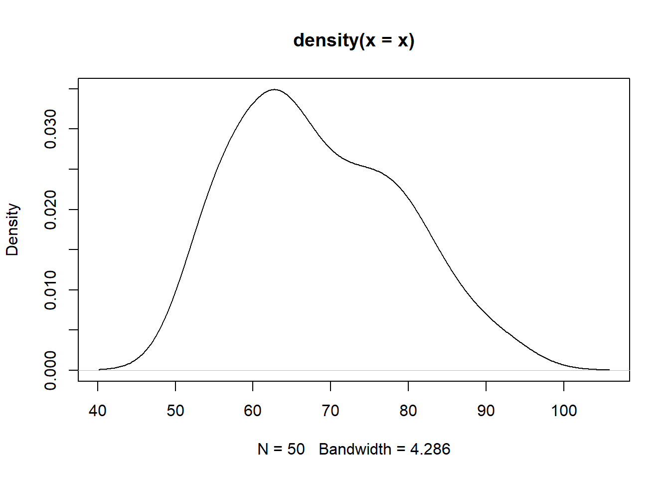
jarque.bera.test(x)##
## Jarque Bera Test
##
## data: x
## X-squared = 2.5432, df = 2, p-value = 0.28043.3. ANOVA
3.3.1. One-way ANOVA (single factor ANOVA)
Please address the lecture for the theory
Example: Investigate good health respondents from depression dataset. Does location affect the results?
# read dataset
Dep = read.table("http://edu.modas.lu/data/txt/depression2.txt",  header=T,  sep="\t",  as.is=FALSE)
str(Dep)
## 'data.frame': 120 obs. of 3 variables:
## $ Location : Factor w/ 3 levels "Florida","New York",..: 1 1 1 1 1 1 1 1 1 1 ...
## $ Health : Factor w/ 2 levels "bad","good": 2 2 2 2 2 2 2 2 2 2 ...
## $ Depression: int 3 7 7 3 8 8 8 5 5 2 ...# consider only healthy
DepGH = Dep[Dep$Health =="good",]
# build 1-way ANOVA model
res1 = aov(Depression ~ Location, DepGH)
summary(res1)## Df Sum Sq Mean Sq F value Pr(>F)
## Location 2 78.5 39.27 6.773 0.0023 **
## Residuals 57 330.4 5.80
## ---
## Signif. codes: 0 '***' 0.001 '**' 0.01 '*' 0.05 '.' 0.1 ' ' 1# add post-hoc analysis
TukeyHSD(res1)## Tukey multiple comparisons of means
## 95% family-wise confidence level
##
## Fit: aov(formula = Depression ~ Location, data = DepGH)
##
## $Location
## diff lwr upr p adj
## New York-Florida 2.8 0.9677423 4.6322577 0.0014973
## North Carolina-Florida 1.5 -0.3322577 3.3322577 0.1289579
## North Carolina-New York -1.3 -3.1322577 0.5322577 0.21126123.3.2. Kruskal-Wallis test
Kruskal-Wallis test is a non-parametric version of one-way ANOVA. Post hoc analysis can be done using pairwise Wilcoxon test or Dunn test.
# non-parametric
kruskal.test(DepGH)
## Warning in kruskal.test.default(DepGH): some elements of 'x' are not numeric
## and will be coerced to numeric##
## Kruskal-Wallis rank sum test
##
## data: DepGH
## Kruskal-Wallis chi-squared = 119, df = 2, p-value < 2.2e-16# posthoc 1
pairwise.wilcox.test(DepGH$Depression, DepGH$Location, p.adjust.method = "bonf")## Warning in wilcox.test.default(xi, xj, paired = paired, ...): cannot compute
## exact p-value with ties## Warning in wilcox.test.default(xi, xj, paired = paired, ...): cannot compute
## exact p-value with ties
## Warning in wilcox.test.default(xi, xj, paired = paired, ...): cannot compute
## exact p-value with ties
##
## Pairwise comparisons using Wilcoxon rank sum test with continuity correction
##
## data: DepGH$Depression and DepGH$Location
##
## Florida New York
## New York 0.0024 -
## North Carolina 0.2137 0.6643
##
## P value adjustment method: bonferroni# posthoc 2
#install.packages("dunn.test")
library(dunn.test)
dunn.test(DepGH$Depression, DepGH$Location)## Kruskal-Wallis rank sum test
##
## data: x and group
## Kruskal-Wallis chi-squared = 10.851, df = 2, p-value = 0
##
##
## Comparison of x by group
## (No adjustment)
## Col Mean-|
## Row Mean | Florida New York
## ---------+----------------------
## New York | -3.276357
## | 0.0005*
## |
## North Ca | -1.933738 1.342619
## | 0.0266 0.0897
##
## alpha = 0.05
## Reject Ho if p <= alpha/23.3.3. Multifactor ANOVA
For the theory - see lecture.
Example - analyze depression from 3 locations and 2 groups of respondents: in good and bad health.
# read dataset
Dep = read.table("http://edu.modas.lu/data/txt/depression2.txt",  header=T,  sep="\t",  as.is=FALSE)
str(Dep)
## 'data.frame': 120 obs. of 3 variables:
## $ Location : Factor w/ 3 levels "Florida","New York",..: 1 1 1 1 1 1 1 1 1 1 ...
## $ Health : Factor w/ 2 levels "bad","good": 2 2 2 2 2 2 2 2 2 2 ...
## $ Depression: int 3 7 7 3 8 8 8 5 5 2 ...boxplot(Depression ~ Health + Location, Dep,las=2,col=c("yellow","cyan"))
# build 2-way ANOVA model
res2 = aov( Depression ~ Health + Location+ Health*Location, Dep)
summary(res2)
## Df Sum Sq Mean Sq F value Pr(>F)
## Health 1 1748.0 1748.0 203.094 <2e-16 ***
## Location 2 73.9 36.9 4.290 0.016 *
## Health:Location 2 26.1 13.1 1.517 0.224
## Residuals 114 981.2 8.6
## ---
## Signif. codes: 0 '***' 0.001 '**' 0.01 '*' 0.05 '.' 0.1 ' ' 1# post-hoc
TukeyHSD(res2)## Tukey multiple comparisons of means
## 95% family-wise confidence level
##
## Fit: aov(formula = Depression ~ Health + Location + Health * Location, data = Dep)
##
## $Health
## diff lwr upr p adj
## good-bad -7.633333 -8.694414 -6.572252 0
##
## $Location
## diff lwr upr p adj
## New York-Florida 1.850 0.2921599 3.4078401 0.0155179
## North Carolina-Florida 0.475 -1.0828401 2.0328401 0.7497611
## North Carolina-New York -1.375 -2.9328401 0.1828401 0.0951631
##
## $`Health:Location`
## diff lwr upr p adj
## good:Florida-bad:Florida -8.95 -11.6393115 -6.260689 0.0000000
## bad:New York-bad:Florida 0.90 -1.7893115 3.589311 0.9264595
## good:New York-bad:Florida -6.15 -8.8393115 -3.460689 0.0000000
## bad:North Carolina-bad:Florida -0.55 -3.2393115 2.139311 0.9913348
## good:North Carolina-bad:Florida -7.45 -10.1393115 -4.760689 0.0000000
## bad:New York-good:Florida 9.85 7.1606885 12.539311 0.0000000
## good:New York-good:Florida 2.80 0.1106885 5.489311 0.0361494
## bad:North Carolina-good:Florida 8.40 5.7106885 11.089311 0.0000000
## good:North Carolina-good:Florida 1.50 -1.1893115 4.189311 0.5892328
## good:New York-bad:New York -7.05 -9.7393115 -4.360689 0.0000000
## bad:North Carolina-bad:New York -1.45 -4.1393115 1.239311 0.6244461
## good:North Carolina-bad:New York -8.35 -11.0393115 -5.660689 0.0000000
## bad:North Carolina-good:New York 5.60 2.9106885 8.289311 0.0000003
## good:North Carolina-good:New York -1.30 -3.9893115 1.389311 0.7262066
## good:North Carolina-bad:North Carolina -6.90 -9.5893115 -4.210689 0.0000000To be square, you could check normaliry of the residuals
shapiro.test( residuals(res2) )##
## Shapiro-Wilk normality test
##
## data: residuals(res2)
## W = 0.98975, p-value = 0.5121Effect size
# get F statistics
FV = anova(res2)$"F value"
FV[length(FV)] = 1
names(FV) = rownames(anova(res2))
barplot(FV, main="F statistics")
abline(h=1,col=2, lty=2)
# get P values
PV = anova(res2)$"Pr(>F)"
PV[length(PV)] = 1
names(PV) = rownames(anova(res2))
barplot(-log10(PV), main="-log10(P-value)")
abline(h=-log10(0.05),col=2, lty=2)
# get sum squares and R2
SS = anova(res2)$"Sum Sq"
names(SS) = rownames(anova(res2))
R2 = SS / sum(SS)
barplot(R2, main="Eta2 (R2) - proportion of variance recovered")
# Cohen's estimation
f = sqrt(R2/(1-R2))
barplot(f, main="Cohen's estimation of effect size")
Example2: Please consider salaries dataset. Build the ANOVA model and interprete.
# read dataset
Sal = read.table("http://edu.modas.lu/data/txt/salaries.txt", header=T,sep="\t",as.is=FALSE)
str(Sal)
## 'data.frame': 30 obs. of 3 variables:
## $ Salary.week: int 872 859 1028 1117 1019 519 702 805 558 591 ...
## $ Occupation : Factor w/ 3 levels "Computer Programmer",..: 2 2 2 2 2 2 2 2 2 2 ...
## $ Gender : Factor w/ 2 levels "Female","Male": 2 2 2 2 2 1 1 1 1 1 ...boxplot(Salary.week ~ Occupation + Gender, Sal, las=2)
# build 2-way ANOVA model
mod = aov(Salary.week ~ Occupation + Gender + Occupation*Gender, Sal)
summary(mod)
## Df Sum Sq Mean Sq F value Pr(>F)
## Occupation 2 276560 138280 13.246 0.000133 ***
## Gender 1 221880 221880 21.254 0.000112 ***
## Occupation:Gender 2 115440 57720 5.529 0.010595 *
## Residuals 24 250552 10440
## ---
## Signif. codes: 0 '***' 0.001 '**' 0.01 '*' 0.05 '.' 0.1 ' ' 1# post-hoc
TukeyHSD(mod)## Tukey multiple comparisons of means
## 95% family-wise confidence level
##
## Fit: aov(formula = Salary.week ~ Occupation + Gender + Occupation * Gender, data = Sal)
##
## $Occupation
## diff lwr upr p adj
## Financial Manager-Computer Programmer 38 -76.11081 152.1108 0.6874260
## Pharmacist-Computer Programmer 220 105.88919 334.1108 0.0001903
## Pharmacist-Financial Manager 182 67.88919 296.1108 0.0015387
##
## $Gender
## diff lwr upr p adj
## Male-Female 172 94.99818 249.0018 0.0001119
##
## $`Occupation:Gender`
## diff lwr upr
## Financial Manager:Female-Computer Programmer:Female -106 -305.80351 93.80351
## Pharmacist:Female-Computer Programmer:Female 190 -9.80351 389.80351
## Computer Programmer:Male-Computer Programmer:Female 56 -143.80351 255.80351
## Financial Manager:Male-Computer Programmer:Female 238 38.19649 437.80351
## Pharmacist:Male-Computer Programmer:Female 306 106.19649 505.80351
## Pharmacist:Female-Financial Manager:Female 296 96.19649 495.80351
## Computer Programmer:Male-Financial Manager:Female 162 -37.80351 361.80351
## Financial Manager:Male-Financial Manager:Female 344 144.19649 543.80351
## Pharmacist:Male-Financial Manager:Female 412 212.19649 611.80351
## Computer Programmer:Male-Pharmacist:Female -134 -333.80351 65.80351
## Financial Manager:Male-Pharmacist:Female 48 -151.80351 247.80351
## Pharmacist:Male-Pharmacist:Female 116 -83.80351 315.80351
## Financial Manager:Male-Computer Programmer:Male 182 -17.80351 381.80351
## Pharmacist:Male-Computer Programmer:Male 250 50.19649 449.80351
## Pharmacist:Male-Financial Manager:Male 68 -131.80351 267.80351
## p adj
## Financial Manager:Female-Computer Programmer:Female 0.5814961
## Pharmacist:Female-Computer Programmer:Female 0.0689592
## Computer Programmer:Male-Computer Programmer:Female 0.9508750
## Financial Manager:Male-Computer Programmer:Female 0.0131635
## Pharmacist:Male-Computer Programmer:Female 0.0010255
## Pharmacist:Female-Financial Manager:Female 0.0015025
## Computer Programmer:Male-Financial Manager:Female 0.1616324
## Financial Manager:Male-Financial Manager:Female 0.0002396
## Pharmacist:Male-Financial Manager:Female 0.0000185
## Computer Programmer:Male-Pharmacist:Female 0.3334443
## Financial Manager:Male-Pharmacist:Female 0.9743050
## Pharmacist:Male-Pharmacist:Female 0.4872344
## Financial Manager:Male-Computer Programmer:Male 0.0889147
## Pharmacist:Male-Computer Programmer:Male 0.0084855
## Pharmacist:Male-Financial Manager:Male 0.89505893.4. LINEAR REGRESSION
3.4.1. Simple linear regression
Dependent variable - the variable that is being predicted or explained. Usually it is denoted by \(y\). Independent variable(s) - the variable(s) that is doing the predicting or explaining. Denoted by \(x\) or \(x_i\).
Example: Cells are grown under different temperature conditions from 20C to 40C. A researched would like to find a dependency between the temperature and the cell number.
Cells = read.table( "http://edu.modas.lu/data/txt/cells.txt",   sep="\t",header=TRUE)
str(Cells)
## 'data.frame': 21 obs. of 2 variables:
## $ Temperature: int 20 21 22 23 24 25 26 27 28 29 ...
## $ Cell.Number: int 83 139 99 143 164 233 198 261 235 264 ...plot(Cells, pch=19)
Regression model. The equation describing how y is related to x and an error term; in simple linear regression, the regression model is \(y = \beta_1 x^2 + \beta_0 + \epsilon\)
Data = read.table("http://edu.modas.lu/data/txt/cells.txt", header=T,sep="\t",quote="\"")
x = Data$Temperature
y = Data$Cell.Number
mod = lm(y~x)
mod
##
## Call:
## lm(formula = y ~ x)
##
## Coefficients:
## (Intercept) x
## -190.78 15.33summary(mod)##
## Call:
## lm(formula = y ~ x)
##
## Residuals:
## Min 1Q Median 3Q Max
## -49.183 -26.190 -1.185 22.147 54.477
##
## Coefficients:
## Estimate Std. Error t value Pr(>|t|)
## (Intercept) -190.784 35.032 -5.446 2.96e-05 ***
## x 15.332 1.145 13.395 3.96e-11 ***
## ---
## Signif. codes: 0 '***' 0.001 '**' 0.01 '*' 0.05 '.' 0.1 ' ' 1
##
## Residual standard error: 31.76 on 19 degrees of freedom
## Multiple R-squared: 0.9042, Adjusted R-squared: 0.8992
## F-statistic: 179.4 on 1 and 19 DF, p-value: 3.958e-11par(mfcol=c(1,2))
# draw the data
plot(x,y,pch=19,main=sprintf("Linear model y(x) = %.1f*x + %.1f",coef(mod)[2],coef(mod)[1]))
# add the regression line and its confidence interval (95%)
lines(x, predict(mod,int = "confidence")[,1],col=2,lwd=2)
lines(x, predict(mod,int = "confidence")[,2],col=2)
lines(x, predict(mod,int = "confidence")[,3],col=2)
# add the prediction interval for the values (95%)
lines(x, predict(mod,int = "pred")[,2],col=4)## Warning in predict.lm(mod, int = "pred"): predictions on current data refer to _future_ responseslines(x, predict(mod,int = "pred")[,3],col=4)## Warning in predict.lm(mod, int = "pred"): predictions on current data refer to _future_ responses## draw residuals
residuals = y - (x*coef(mod)[2] + coef(mod)[1])
plot(x, residuals,pch=19,main="Residuals")
abline(h=0,col=2,lwd=2)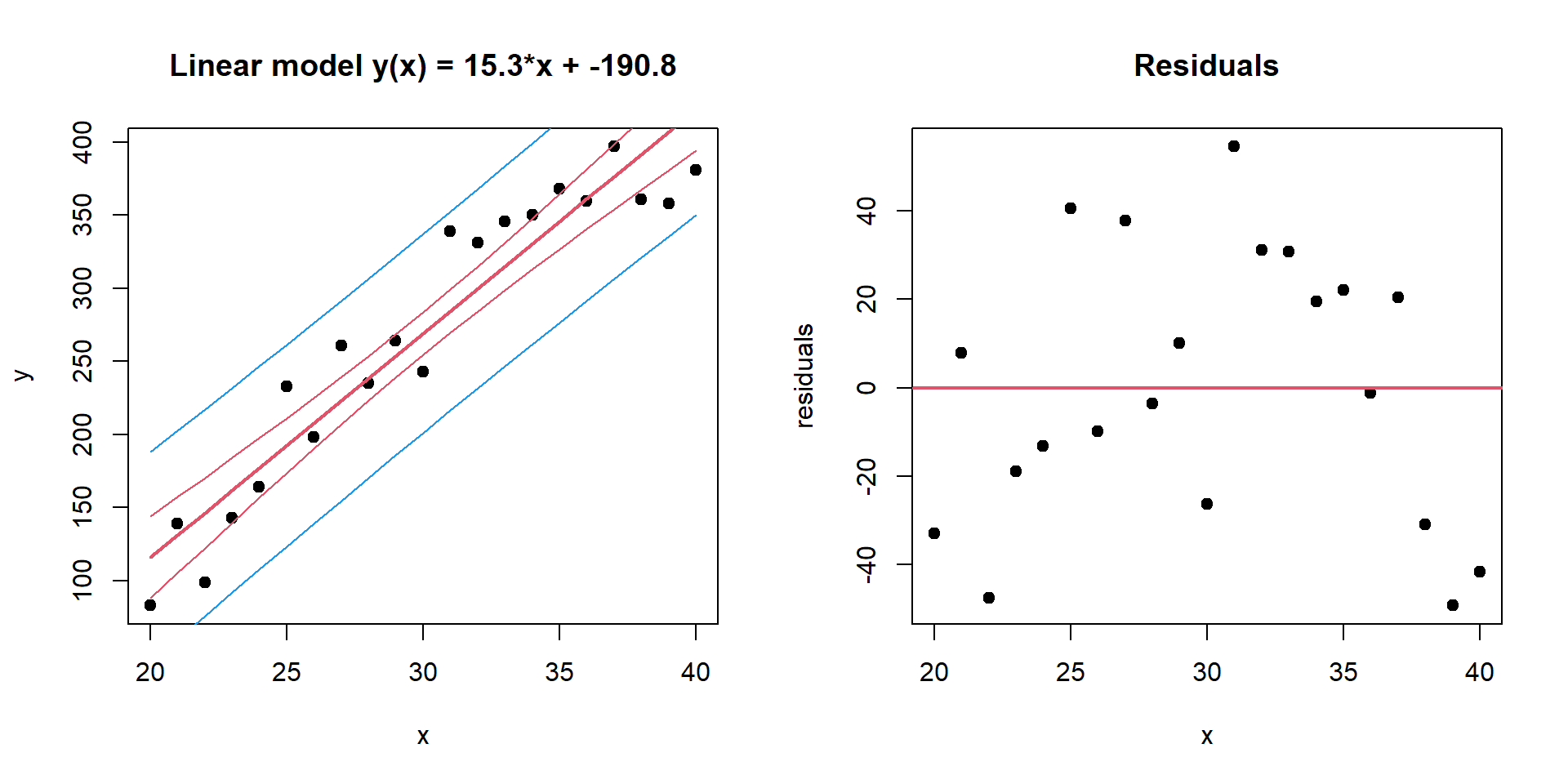
Now, let’s predict how many cells we should expect under Temperature = \(37^\circ\)C.
## confidence (where the mean will be)
predict(mod,data.frame(x=37),int = "confidence")
## fit lwr upr
## 1 376.5177 354.3436 398.6919## prediction (where the actual observation will be)
predict(mod,data.frame(x=37),int = "pred")## fit lwr upr
## 1 376.5177 306.4377 446.59783.4.2. Multiple linear regression
Often one variable is not enough, and we need several independent
variables to predict dependent one. Let’s consider internal
swiss dataset: standardized fertility measure and
socio-economic indicators for 47 French-speaking provinces of
Switzerland at about 1888. See ?swiss
str(swiss)## 'data.frame': 47 obs. of 6 variables:
## $ Fertility : num 80.2 83.1 92.5 85.8 76.9 76.1 83.8 92.4 82.4 82.9 ...
## $ Agriculture : num 17 45.1 39.7 36.5 43.5 35.3 70.2 67.8 53.3 45.2 ...
## $ Examination : int 15 6 5 12 17 9 16 14 12 16 ...
## $ Education : int 12 9 5 7 15 7 7 8 7 13 ...
## $ Catholic : num 9.96 84.84 93.4 33.77 5.16 ...
## $ Infant.Mortality: num 22.2 22.2 20.2 20.3 20.6 26.6 23.6 24.9 21 24.4 ...## overview of the data
#install.packages("PerformanceAnalytics")
library(PerformanceAnalytics)## Warning: package 'PerformanceAnalytics' was built under R version 4.3.3## Loading required package: xts## Warning: package 'xts' was built under R version 4.3.3## Loading required package: zoo##
## Attaching package: 'zoo'## The following objects are masked from 'package:base':
##
## as.Date, as.Date.numeric##
## Attaching package: 'PerformanceAnalytics'## The following object is masked from 'package:graphics':
##
## legendchart.Correlation(swiss)## Warning in par(usr): argument 1 does not name a graphical parameter## Warning in par(usr): argument 1 does not name a graphical parameter
## Warning in par(usr): argument 1 does not name a graphical parameter
## Warning in par(usr): argument 1 does not name a graphical parameter
## Warning in par(usr): argument 1 does not name a graphical parameter
## Warning in par(usr): argument 1 does not name a graphical parameter
## Warning in par(usr): argument 1 does not name a graphical parameter
## Warning in par(usr): argument 1 does not name a graphical parameter
## Warning in par(usr): argument 1 does not name a graphical parameter
## Warning in par(usr): argument 1 does not name a graphical parameter
## Warning in par(usr): argument 1 does not name a graphical parameter
## Warning in par(usr): argument 1 does not name a graphical parameter
## Warning in par(usr): argument 1 does not name a graphical parameter
## Warning in par(usr): argument 1 does not name a graphical parameter
## Warning in par(usr): argument 1 does not name a graphical parameter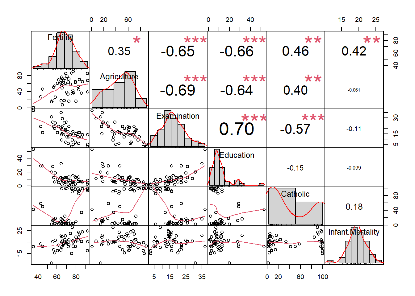
## see complete model
modAll = lm(Fertility ~ . , data = swiss)
summary(modAll)##
## Call:
## lm(formula = Fertility ~ ., data = swiss)
##
## Residuals:
## Min 1Q Median 3Q Max
## -15.2743 -5.2617 0.5032 4.1198 15.3213
##
## Coefficients:
## Estimate Std. Error t value Pr(>|t|)
## (Intercept) 66.91518 10.70604 6.250 1.91e-07 ***
## Agriculture -0.17211 0.07030 -2.448 0.01873 *
## Examination -0.25801 0.25388 -1.016 0.31546
## Education -0.87094 0.18303 -4.758 2.43e-05 ***
## Catholic 0.10412 0.03526 2.953 0.00519 **
## Infant.Mortality 1.07705 0.38172 2.822 0.00734 **
## ---
## Signif. codes: 0 '***' 0.001 '**' 0.01 '*' 0.05 '.' 0.1 ' ' 1
##
## Residual standard error: 7.165 on 41 degrees of freedom
## Multiple R-squared: 0.7067, Adjusted R-squared: 0.671
## F-statistic: 19.76 on 5 and 41 DF, p-value: 5.594e-10## remove correlated & non-significant variable... not really correct
modSig = lm(Fertility ~ . - Examination , data = swiss)
summary(modSig)##
## Call:
## lm(formula = Fertility ~ . - Examination, data = swiss)
##
## Residuals:
## Min 1Q Median 3Q Max
## -14.6765 -6.0522 0.7514 3.1664 16.1422
##
## Coefficients:
## Estimate Std. Error t value Pr(>|t|)
## (Intercept) 62.10131 9.60489 6.466 8.49e-08 ***
## Agriculture -0.15462 0.06819 -2.267 0.02857 *
## Education -0.98026 0.14814 -6.617 5.14e-08 ***
## Catholic 0.12467 0.02889 4.315 9.50e-05 ***
## Infant.Mortality 1.07844 0.38187 2.824 0.00722 **
## ---
## Signif. codes: 0 '***' 0.001 '**' 0.01 '*' 0.05 '.' 0.1 ' ' 1
##
## Residual standard error: 7.168 on 42 degrees of freedom
## Multiple R-squared: 0.6993, Adjusted R-squared: 0.6707
## F-statistic: 24.42 on 4 and 42 DF, p-value: 1.717e-10## make simple regression using the most significant variable
mod1 = lm(Fertility ~ Education , data = swiss)
summary(mod1)##
## Call:
## lm(formula = Fertility ~ Education, data = swiss)
##
## Residuals:
## Min 1Q Median 3Q Max
## -17.036 -6.711 -1.011 9.526 19.689
##
## Coefficients:
## Estimate Std. Error t value Pr(>|t|)
## (Intercept) 79.6101 2.1041 37.836 < 2e-16 ***
## Education -0.8624 0.1448 -5.954 3.66e-07 ***
## ---
## Signif. codes: 0 '***' 0.001 '**' 0.01 '*' 0.05 '.' 0.1 ' ' 1
##
## Residual standard error: 9.446 on 45 degrees of freedom
## Multiple R-squared: 0.4406, Adjusted R-squared: 0.4282
## F-statistic: 35.45 on 1 and 45 DF, p-value: 3.659e-07## Let's remove correlated features by PCA
PC = prcomp(swiss[,-1])
swiss2 = data.frame(Fertility = swiss$Fertility, PC$x)
chart.Correlation(swiss2)## Warning in par(usr): argument 1 does not name a graphical parameter
## Warning in par(usr): argument 1 does not name a graphical parameter

## Warning in par(usr): argument 1 does not name a graphical parameter

## Warning in par(usr): argument 1 does not name a graphical parameter

## Warning in par(usr): argument 1 does not name a graphical parameter

## Warning in par(usr): argument 1 does not name a graphical parameter

## Warning in par(usr): argument 1 does not name a graphical parameter

## Warning in par(usr): argument 1 does not name a graphical parameter

## Warning in par(usr): argument 1 does not name a graphical parameter

## Warning in par(usr): argument 1 does not name a graphical parameter

## Warning in par(usr): argument 1 does not name a graphical parameter

## Warning in par(usr): argument 1 does not name a graphical parameter

## Warning in par(usr): argument 1 does not name a graphical parameter

## Warning in par(usr): argument 1 does not name a graphical parameter

## Warning in par(usr): argument 1 does not name a graphical parameter
modPC = lm(Fertility ~ ., data = swiss2)
summary(modPC)
##
## Call:
## lm(formula = Fertility ~ ., data = swiss2)
##
## Residuals:
## Min 1Q Median 3Q Max
## -15.2743 -5.2617 0.5032 4.1198 15.3213
##
## Coefficients:
## Estimate Std. Error t value Pr(>|t|)
## (Intercept) 70.14255 1.04518 67.111 < 2e-16 ***
## PC1 0.14376 0.02437 5.900 6.00e-07 ***
## PC2 -0.11115 0.04930 -2.255 0.0296 *
## PC3 0.98882 0.13774 7.179 9.23e-09 ***
## PC4 -0.29483 0.28341 -1.040 0.3043
## PC5 -0.96327 0.38410 -2.508 0.0162 *
## ---
## Signif. codes: 0 '***' 0.001 '**' 0.01 '*' 0.05 '.' 0.1 ' ' 1
##
## Residual standard error: 7.165 on 41 degrees of freedom
## Multiple R-squared: 0.7067, Adjusted R-squared: 0.671
## F-statistic: 19.76 on 5 and 41 DF, p-value: 5.594e-10modPCSig = lm(Fertility ~ .-PC4, data = swiss2)
summary(modPCSig)##
## Call:
## lm(formula = Fertility ~ . - PC4, data = swiss2)
##
## Residuals:
## Min 1Q Median 3Q Max
## -16.276 -3.959 -0.651 4.519 14.416
##
## Coefficients:
## Estimate Std. Error t value Pr(>|t|)
## (Intercept) 70.14255 1.04620 67.045 < 2e-16 ***
## PC1 0.14376 0.02439 5.895 5.63e-07 ***
## PC2 -0.11115 0.04934 -2.253 0.0296 *
## PC3 0.98882 0.13788 7.172 8.26e-09 ***
## PC5 -0.96327 0.38448 -2.505 0.0162 *
## ---
## Signif. codes: 0 '***' 0.001 '**' 0.01 '*' 0.05 '.' 0.1 ' ' 1
##
## Residual standard error: 7.172 on 42 degrees of freedom
## Multiple R-squared: 0.699, Adjusted R-squared: 0.6703
## F-statistic: 24.38 on 4 and 42 DF, p-value: 1.76e-10How to choose the proper model? Several approaches:
maximizing adjusted R2
Add / remove variable and compare models using likelihood ratio or chi2 test.
## calculate AIC and select minimal AIC
AIC(mod1,modSig, modAll, modPC, modPCSig)
## df AIC
## mod1 3 348.4223
## modSig 6 325.2408
## modAll 7 326.0716
## modPC 7 326.0716
## modPCSig 6 325.2961BIC(mod1,modSig, modAll, modPC, modPCSig)## df BIC
## mod1 3 353.9727
## modSig 6 336.3417
## modAll 7 339.0226
## modPC 7 339.0226
## modPCSig 6 336.3970## Is fitting significantly better? Likelihood
anova(modAll,modSig)## Analysis of Variance Table
##
## Model 1: Fertility ~ Agriculture + Examination + Education + Catholic +
## Infant.Mortality
## Model 2: Fertility ~ (Agriculture + Examination + Education + Catholic +
## Infant.Mortality) - Examination
## Res.Df RSS Df Sum of Sq F Pr(>F)
## 1 41 2105.0
## 2 42 2158.1 -1 -53.027 1.0328 0.3155anova(modAll,mod1)## Analysis of Variance Table
##
## Model 1: Fertility ~ Agriculture + Examination + Education + Catholic +
## Infant.Mortality
## Model 2: Fertility ~ Education
## Res.Df RSS Df Sum of Sq F Pr(>F)
## 1 41 2105.0
## 2 45 4015.2 -4 -1910.2 9.3012 1.916e-05 ***
## ---
## Signif. codes: 0 '***' 0.001 '**' 0.01 '*' 0.05 '.' 0.1 ' ' 1## this is not very informative (use training set)
plot(swiss$Fertility, predict(modAll,swiss),xlab="Real Fertility",ylab="Predicted Fertility",pch=19)
abline(a=0,b=1,col=2,lty=2)
| Prev Home Next |
By Petr Nazarov
|