Lecture 4. Advanced topics
Petr V. Nazarov, LIH
2024-04-08
| Materials: Video Tasks |
4.1. ADVANCED REGRESSION
Some classical definitions regarding regression. Please note that in the literature last 15 years these terms are often mixed. Do not be surprised… :)
\[ y = function(x) \]
Univariable or “simple” model - is a model with a single independent variable (for each observation, x is a scalar)
Univariate - is a model with a single dependent variable (for each observation, y is a scalar)
Multivariable - is a model with several independent variables (for each observation, x is a vector)
Multivariate - is a model with several dependent variables (for each observation, y is a vector)
4.1.1. Linear regression with categorical variables
Example: The MASS::birthwt data frame
has 189 rows and 10 columns. The data were collected at Baystate Medical
Center, Springfield, Mass, during 1986. The dataframe includes the
following parameters (slightly modified for this course):
low - indicator of birth weight less than 2.5 kg (yes/no)
age - mother’s age in years
mwt - mother’s weight in kg at last menstrual period
race - mother’s race
smoke - smoking status during pregnancy
ptl - number of previous premature labors
ht - history of hypertension
ui - presence of uterine irritability
ftv - number of physician visits during the first trimester
bwt - birth weight in grams
Let’s import the data
BWT = read.table("http://edu.modas.lu/data/txt/birthwt.txt",header=TRUE, sep="\t",comment.char="#",as.is=FALSE)
str(BWT)
## 'data.frame': 189 obs. of 10 variables:
## $ low : Factor w/ 2 levels "no","yes": 1 1 1 1 1 1 1 1 1 1 ...
## $ age : int 19 33 20 21 18 21 22 17 29 26 ...
## $ mwt : num 82.6 70.3 47.6 49 48.5 56.2 53.5 46.7 55.8 51.3 ...
## $ race : Factor w/ 3 levels "black","other",..: 1 2 3 3 3 2 3 2 3 3 ...
## $ smoke: Factor w/ 2 levels "no","yes": 1 1 2 2 2 1 1 1 2 2 ...
## $ ptl : int 0 0 0 0 0 0 0 0 0 0 ...
## $ ht : Factor w/ 2 levels "no","yes": 1 1 1 1 1 1 1 1 1 1 ...
## $ ui : Factor w/ 2 levels "no","yes": 2 1 1 2 2 1 1 1 1 1 ...
## $ ftv : int 0 3 1 2 0 0 1 1 1 0 ...
## $ bwt : int 2523 2551 2557 2594 2600 2622 2637 2637 2663 2665 ...Let’s fit simple linear regression model: \[ y = \beta_0 + \beta_1 \times x\] where y
- bwt (child birth weight), x - mwt (mother
weight)
# Fit regression model
mod1 = lm(bwt ~ mwt, data = BWT)
summary(mod1)
##
## Call:
## lm(formula = bwt ~ mwt, data = BWT)
##
## Residuals:
## Min 1Q Median 3Q Max
## -2191.77 -498.28 -3.57 508.40 2075.55
##
## Coefficients:
## Estimate Std. Error t value Pr(>|t|)
## (Intercept) 2369.252 228.502 10.369 <2e-16 ***
## mwt 9.771 3.778 2.586 0.0105 *
## ---
## Signif. codes: 0 '***' 0.001 '**' 0.01 '*' 0.05 '.' 0.1 ' ' 1
##
## Residual standard error: 718.4 on 187 degrees of freedom
## Multiple R-squared: 0.03454, Adjusted R-squared: 0.02937
## F-statistic: 6.689 on 1 and 187 DF, p-value: 0.01046library(ggplot2)
p = ggplot(BWT, aes(x = mwt, y = bwt)) +
geom_point(aes(color = race, shape = smoke)) + stat_smooth(method = "lm", color = 1)
print(p)## `geom_smooth()` using formula = 'y ~ x'
Now we will add categorical variable: smoke. So, we use
following regression:
\[ bwt = \beta_{0, smoke} + \beta_1 \times mwt\]
mod2 = lm(bwt ~ mwt + smoke, data = BWT)
summary(mod2)
##
## Call:
## lm(formula = bwt ~ mwt + smoke, data = BWT)
##
## Residuals:
## Min 1Q Median 3Q Max
## -2031.17 -445.85 29.17 521.73 1967.73
##
## Coefficients:
## Estimate Std. Error t value Pr(>|t|)
## (Intercept) 2500.872 230.860 10.833 <2e-16 ***
## mwt 9.344 3.726 2.508 0.0130 *
## smokeyes -272.005 105.591 -2.576 0.0108 *
## ---
## Signif. codes: 0 '***' 0.001 '**' 0.01 '*' 0.05 '.' 0.1 ' ' 1
##
## Residual standard error: 707.8 on 186 degrees of freedom
## Multiple R-squared: 0.0678, Adjusted R-squared: 0.05777
## F-statistic: 6.763 on 2 and 186 DF, p-value: 0.001461# Calculate smoke-specific intercepts
intercepts = c(coef(mod2)["(Intercept)"],
coef(mod2)["(Intercept)"] + coef(mod2)["smokeyes"])
# Create dataframe with regression coefficients
lines_df = data.frame(intercepts = intercepts,
slopes = rep(coef(mod2)["mwt"], 2),
smoke = levels(BWT$smoke))
qplot(x = mwt, y = bwt, color = smoke, data = BWT) +
geom_abline(aes(intercept = intercepts,
slope = slopes,
color = smoke), data = lines_df)## Warning: `qplot()` was deprecated in ggplot2 3.4.0.
## This warning is displayed once every 8 hours.
## Call `lifecycle::last_lifecycle_warnings()` to see where this warning was
## generated.
We can do the same with race:
\[ bwt = \beta_{0,race} + \beta_1 \times mwt\] Please note, how intercepts are calculated now (“race black” is considered as reference!):
mod3 = lm(bwt ~ mwt + race, data = BWT)
summary(mod3)
##
## Call:
## lm(formula = bwt ~ mwt + race, data = BWT)
##
## Residuals:
## Min 1Q Median 3Q Max
## -2095.88 -419.18 41.79 478.29 1929.45
##
## Coefficients:
## Estimate Std. Error t value Pr(>|t|)
## (Intercept) 2034.454 291.619 6.976 5.22e-11 ***
## mwt 10.289 3.859 2.667 0.00834 **
## raceother 210.684 169.079 1.246 0.21432
## racewhite 451.948 157.565 2.868 0.00461 **
## ---
## Signif. codes: 0 '***' 0.001 '**' 0.01 '*' 0.05 '.' 0.1 ' ' 1
##
## Residual standard error: 703 on 185 degrees of freedom
## Multiple R-squared: 0.08533, Adjusted R-squared: 0.0705
## F-statistic: 5.753 on 3 and 185 DF, p-value: 0.0008766# Calculate race-specific intercepts
intercepts = c(coef(mod3)["(Intercept)"],
coef(mod3)["(Intercept)"] + coef(mod3)["raceother"],
coef(mod3)["(Intercept)"] + coef(mod3)["racewhite"])
# Create dataframe with regression coefficients
lines_df = data.frame(intercepts = intercepts,
slopes = rep(coef(mod2)["mwt"], 3),
race = levels(BWT$race))
qplot(x = mwt, y = bwt, color = race, data = BWT) +
geom_abline(aes(intercept = intercepts,
slope = slopes,
color = race), data = lines_df)
Next, we could allow slope coefficients to change as well. This will be equivalent to interactions.
\[ bwt = \beta_{0,smoke} + \beta_{1,smoke} \times mwt\]
mod4 = lm(bwt ~ mwt + smoke + mwt*smoke, data = BWT)
summary(mod4)
##
## Call:
## lm(formula = bwt ~ mwt + smoke + mwt * smoke, data = BWT)
##
## Residuals:
## Min 1Q Median 3Q Max
## -2038.59 -454.86 28.28 530.79 1976.79
##
## Coefficients:
## Estimate Std. Error t value Pr(>|t|)
## (Intercept) 2350.577 312.762 7.516 2.36e-12 ***
## mwt 11.875 5.148 2.307 0.0222 *
## smokeyes 40.929 451.209 0.091 0.9278
## mwt:smokeyes -5.330 7.471 -0.713 0.4765
## ---
## Signif. codes: 0 '***' 0.001 '**' 0.01 '*' 0.05 '.' 0.1 ' ' 1
##
## Residual standard error: 708.8 on 185 degrees of freedom
## Multiple R-squared: 0.07035, Adjusted R-squared: 0.05528
## F-statistic: 4.667 on 3 and 185 DF, p-value: 0.003617# Calculate smoke-specific intercepts
intercepts = c(coef(mod4)["(Intercept)"],
coef(mod4)["(Intercept)"] + coef(mod4)["smokeyes"])
# Calculate smoke-specific slopes
slopes = c(coef(mod4)["mwt"],
coef(mod4)["mwt"] + coef(mod4)["mwt:smokeyes"])
# Create dataframe with regression coefficients
lines_df = data.frame(intercepts = intercepts,
slopes = slopes,
smoke = levels(BWT$smoke))
qplot(x = mwt, y = bwt, color = smoke, data = BWT) +
geom_abline(aes(intercept = intercepts,
slope = slopes,
color = smoke), data = lines_df)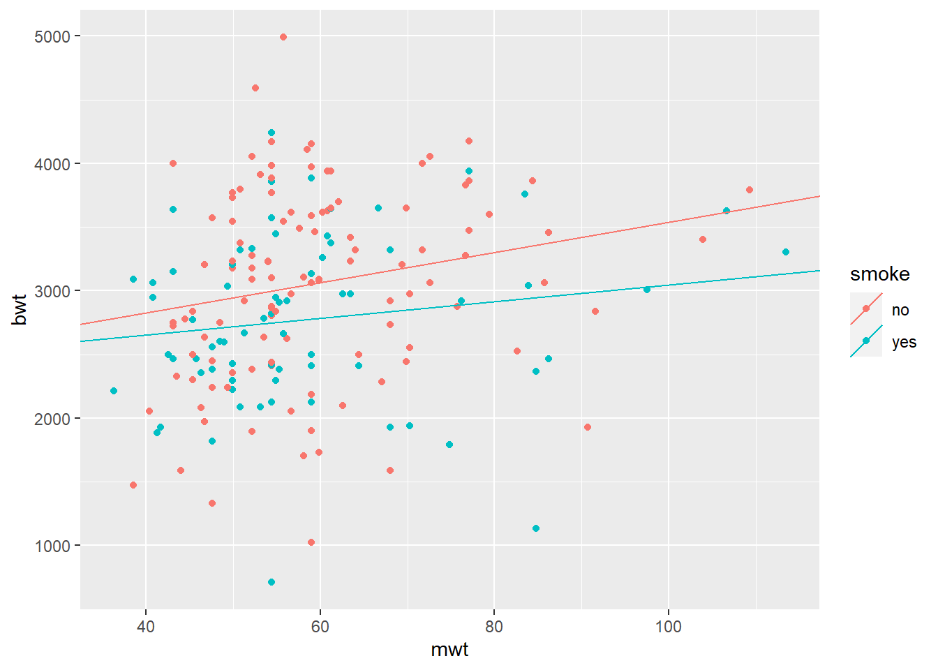
Same for race: \[ bwt = \beta_{0,race} +
\beta_{1,race} \times mwt\] See the loss of significance in
mod5 compared to mod3
mod5 = lm(bwt ~ mwt + race + mwt*race, data = BWT)
summary(mod5)
##
## Call:
## lm(formula = bwt ~ mwt + race + mwt * race, data = BWT)
##
## Residuals:
## Min 1Q Median 3Q Max
## -2095.76 -450.39 55.81 493.18 1932.46
##
## Coefficients:
## Estimate Std. Error t value Pr(>|t|)
## (Intercept) 2362.268 540.948 4.367 2.11e-05 ***
## mwt 5.367 7.852 0.683 0.495
## raceother -292.398 687.153 -0.426 0.671
## racewhite 80.144 637.041 0.126 0.900
## mwt:raceother 8.142 10.943 0.744 0.458
## mwt:racewhite 5.657 9.579 0.591 0.556
## ---
## Signif. codes: 0 '***' 0.001 '**' 0.01 '*' 0.05 '.' 0.1 ' ' 1
##
## Residual standard error: 705.7 on 183 degrees of freedom
## Multiple R-squared: 0.08827, Adjusted R-squared: 0.06336
## F-statistic: 3.543 on 5 and 183 DF, p-value: 0.00441# Calculate smoke-specific intercepts
intercepts = c(coef(mod5)["(Intercept)"],
coef(mod5)["(Intercept)"] + coef(mod5)["raceother"],
coef(mod5)["(Intercept)"] + coef(mod5)["racewhite"])
# Calculate smoke-specific slopes
slopes = c(coef(mod5)["mwt"],
coef(mod5)["mwt"] + coef(mod5)["mwt:raceother"],
coef(mod5)["mwt"] + coef(mod5)["mwt:racewhite"])
# Create dataframe with regression coefficients
lines_df = data.frame(intercepts = intercepts,
slopes = slopes,
race = levels(BWT$race))
qplot(x = mwt, y = bwt, color = race, data = BWT) +
geom_abline(aes(intercept = intercepts,
slope = slopes,
color = race), data = lines_df)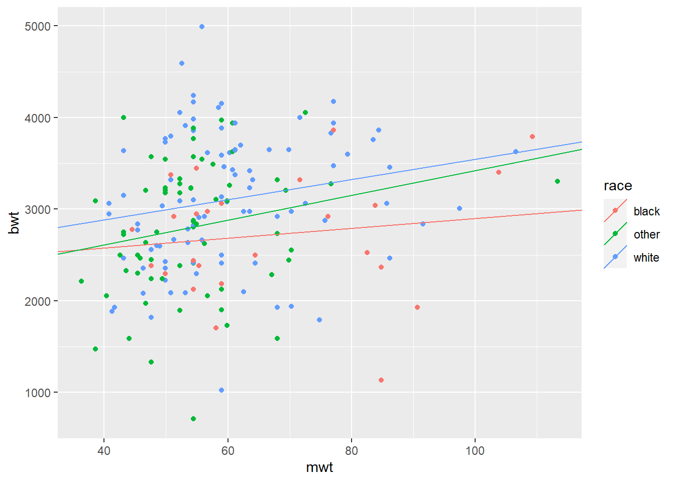
Check all variables and select significant:
## all variables
mod5 = lm(bwt ~ ., data = BWT[,-1])
summary(mod5)
##
## Call:
## lm(formula = bwt ~ ., data = BWT[, -1])
##
## Residuals:
## Min 1Q Median 3Q Max
## -1825.43 -435.47 55.48 473.21 1701.23
##
## Coefficients:
## Estimate Std. Error t value Pr(>|t|)
## (Intercept) 2438.861 327.262 7.452 3.77e-12 ***
## age -3.571 9.620 -0.371 0.71093
## mwt 9.609 3.826 2.511 0.01292 *
## raceother 133.531 159.396 0.838 0.40330
## racewhite 488.522 149.982 3.257 0.00135 **
## smokeyes -351.920 106.476 -3.305 0.00115 **
## ptl -48.454 101.965 -0.475 0.63522
## htyes -592.964 202.316 -2.931 0.00382 **
## uiyes -516.139 138.878 -3.716 0.00027 ***
## ftv -14.083 46.467 -0.303 0.76218
## ---
## Signif. codes: 0 '***' 0.001 '**' 0.01 '*' 0.05 '.' 0.1 ' ' 1
##
## Residual standard error: 650.3 on 179 degrees of freedom
## Multiple R-squared: 0.2428, Adjusted R-squared: 0.2047
## F-statistic: 6.377 on 9 and 179 DF, p-value: 7.849e-08## significant variables
mod6 = lm(bwt ~ mwt + race + smoke + ht + ui, data = BWT[,-1])
summary(mod6)##
## Call:
## lm(formula = bwt ~ mwt + race + smoke + ht + ui, data = BWT[,
## -1])
##
## Residuals:
## Min 1Q Median 3Q Max
## -1842.33 -432.72 67.34 459.25 1631.03
##
## Coefficients:
## Estimate Std. Error t value Pr(>|t|)
## (Intercept) 2361.538 281.653 8.385 1.36e-14 ***
## mwt 9.360 3.694 2.534 0.012121 *
## raceother 127.078 157.597 0.806 0.421094
## racewhite 475.142 145.600 3.263 0.001315 **
## smokeyes -356.207 103.444 -3.443 0.000713 ***
## htyes -585.313 199.640 -2.932 0.003802 **
## uiyes -525.592 134.667 -3.903 0.000134 ***
## ---
## Signif. codes: 0 '***' 0.001 '**' 0.01 '*' 0.05 '.' 0.1 ' ' 1
##
## Residual standard error: 645.9 on 182 degrees of freedom
## Multiple R-squared: 0.2404, Adjusted R-squared: 0.2154
## F-statistic: 9.602 on 6 and 182 DF, p-value: 3.582e-094.1.2. Logistic regression
Now let’s try to predict underweight in children on the same data. Logistic regression fits the following function (linear function warped in a sigmoid).
\[ y = \frac{1}{1+e^{-(\beta_0+\beta_1x_1+\beta_2x_2+...)}} = \frac{e^{\beta_0+\beta_1x_1+\beta_2x_2+...}}{1+e^{\beta_0+\beta_1x_1+\beta_2x_2+...}}\] where \(y \in [0,1]\)
Column low shows when the weight is below 2500g. Let’s
create a new variable outcome, with outcome=0 for
underweight kids and Y=1 for normal weight (it is inverted
low, but will be easier for interpretation afterwards). We
should also replace “no” with 0 and “yes” with 1 in all factors. For
factors that have more than 2 levels, use “dummy” variables :)
BWT2 = BWT ## create a new data frame
## dummy variable for race: default will be "other"
BWT2$raceblack = as.integer(BWT2$race == "black")
BWT2$racewhite = as.integer(BWT2$race == "white")
BWT2$smoke = as.integer(BWT2$smoke == "yes")
BWT2$ht = as.integer(BWT2$ht == "yes")
BWT2$ui = as.integer(BWT2$ui == "yes")
BWT2$outcome = as.integer(BWT2$low == "no")
## remove not needed columns to avoid info leackage
BWT2$low = NULL
BWT2$bwt = NULL
BWT2$race = NULL
str(BWT2)
## 'data.frame': 189 obs. of 10 variables:
## $ age : int 19 33 20 21 18 21 22 17 29 26 ...
## $ mwt : num 82.6 70.3 47.6 49 48.5 56.2 53.5 46.7 55.8 51.3 ...
## $ smoke : int 0 0 1 1 1 0 0 0 1 1 ...
## $ ptl : int 0 0 0 0 0 0 0 0 0 0 ...
## $ ht : int 0 0 0 0 0 0 0 0 0 0 ...
## $ ui : int 1 0 0 1 1 0 0 0 0 0 ...
## $ ftv : int 0 3 1 2 0 0 1 1 1 0 ...
## $ raceblack: int 1 0 0 0 0 0 0 0 0 0 ...
## $ racewhite: int 0 0 1 1 1 0 1 0 1 1 ...
## $ outcome : int 1 1 1 1 1 1 1 1 1 1 ...Now let’s see the global model (multivariable):
logmod1 = glm(outcome ~ .,family = "binomial", data = BWT2)
summary(logmod1)
##
## Call:
## glm(formula = outcome ~ ., family = "binomial", data = BWT2)
##
## Coefficients:
## Estimate Std. Error z value Pr(>|z|)
## (Intercept) -1.36253 1.10477 -1.233 0.21745
## age 0.02955 0.03703 0.798 0.42483
## mwt 0.03403 0.01526 2.230 0.02572 *
## smoke -0.93838 0.40216 -2.333 0.01963 *
## ptl -0.54362 0.34541 -1.574 0.11552
## ht -1.86375 0.69759 -2.672 0.00755 **
## ui -0.76787 0.45933 -1.672 0.09458 .
## ftv -0.06537 0.17240 -0.379 0.70455
## raceblack -0.39230 0.53768 -0.730 0.46562
## racewhite 0.88022 0.44080 1.997 0.04584 *
## ---
## Signif. codes: 0 '***' 0.001 '**' 0.01 '*' 0.05 '.' 0.1 ' ' 1
##
## (Dispersion parameter for binomial family taken to be 1)
##
## Null deviance: 234.67 on 188 degrees of freedom
## Residual deviance: 201.28 on 179 degrees of freedom
## AIC: 221.28
##
## Number of Fisher Scoring iterations: 4And only significant
logmod2 = glm(outcome ~ mwt + smoke + ht + ui + racewhite,family = "binomial", data = BWT2)
summary(logmod2)
##
## Call:
## glm(formula = outcome ~ mwt + smoke + ht + ui + racewhite, family = "binomial",
## data = BWT2)
##
## Coefficients:
## Estimate Std. Error z value Pr(>|z|)
## (Intercept) -0.90549 0.83782 -1.081 0.27980
## mwt 0.03371 0.01423 2.369 0.01786 *
## smoke -1.09082 0.38661 -2.822 0.00478 **
## ht -1.85349 0.68827 -2.693 0.00708 **
## ui -0.89284 0.44952 -1.986 0.04701 *
## racewhite 1.06467 0.38811 2.743 0.00608 **
## ---
## Signif. codes: 0 '***' 0.001 '**' 0.01 '*' 0.05 '.' 0.1 ' ' 1
##
## (Dispersion parameter for binomial family taken to be 1)
##
## Null deviance: 234.67 on 188 degrees of freedom
## Residual deviance: 204.76 on 183 degrees of freedom
## AIC: 216.76
##
## Number of Fisher Scoring iterations: 4Res = data.frame(Labels = names(coef(logmod1)))
Res$LogOdds = coef(logmod1)
Res$LogOdds1 = confint(logmod1)[,1]## Waiting for profiling to be done...Res$LogOdds2 = confint(logmod1)[,2]## Waiting for profiling to be done...(p <- ggplot(Res, aes(x = LogOdds, y = Labels)) +
geom_vline(aes(xintercept = 0), size = .25, linetype = 'dashed') +
geom_errorbarh(aes(xmax = LogOdds2, xmin = LogOdds1), linewidth = 0.5, height = 0.2, color = 'gray50') +
geom_point(size = 3.5, color = 'orange') +
theme_bw() +
theme(panel.grid.minor = element_blank()) +
scale_x_continuous(breaks = seq(-5,5,1) ) +
ylab('') +
xlab('Odds ratio (log scale)') +
ggtitle('Multivariable Model')
)## Warning: Using `size` aesthetic for lines was deprecated in ggplot2 3.4.0.
## ℹ Please use `linewidth` instead.
## This warning is displayed once every 8 hours.
## Call `lifecycle::last_lifecycle_warnings()` to see where this warning was
## generated.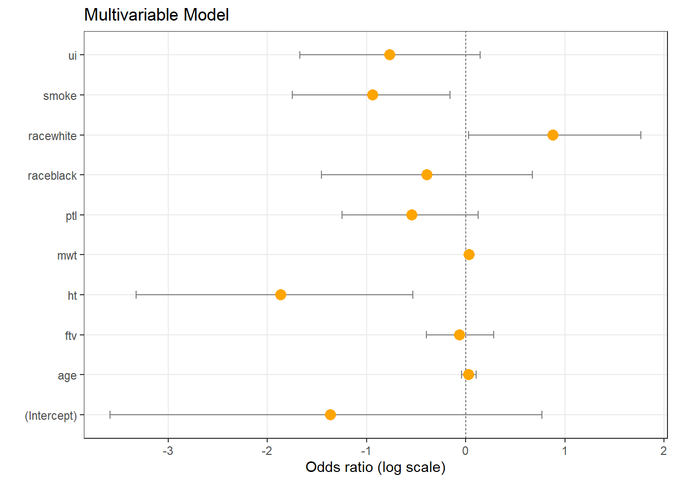
Interpretation: smoke is significantly linked to weight (lowering weight if smoke=1). racewhite positively linked to weight (increasing weight in racewhite=1), etc.
Feel free to repeat this analysis using set of univariable models :)
4.2. SURVIVAL ANALYSIS
4.2.1. Definitions, Kaplan-Meier plot
Survival analysis is a branch of statistics which deals with analysis of time to events, such as death in biological organisms and failure in mechanical systems (i.e. reliability theory in engineering).
Survival analysis attempts to answer questions such as:
What is the proportion of a population which will survive past a certain time?
Of those that survive, at what rate will they die or fail?
Can multiple causes of death or failure be taken into account?
How do particular circumstances or characteristics increase or decrease the probability of survival?
Survival data include:
Time-to-event: The duration from the start of the study until an event of interest occurs (such as death) or until the subject is censored (for example, if the patient withdraws from the study).
Censoring status: A variable indicating whether the endpoint was observed (1 for the event occurrence) or censored (0 for non-occurrence due to end of study period or withdrawal).
Predictor variables: Various factors or covariates that may influence the time to the event, which can be continuous or categorical in nature.
library(survival)
str(lung)
## 'data.frame': 228 obs. of 10 variables:
## $ inst : num 3 3 3 5 1 12 7 11 1 7 ...
## $ time : num 306 455 1010 210 883 ...
## $ status : num 2 2 1 2 2 1 2 2 2 2 ...
## $ age : num 74 68 56 57 60 74 68 71 53 61 ...
## $ sex : num 1 1 1 1 1 1 2 2 1 1 ...
## $ ph.ecog : num 1 0 0 1 0 1 2 2 1 2 ...
## $ ph.karno : num 90 90 90 90 100 50 70 60 70 70 ...
## $ pat.karno: num 100 90 90 60 90 80 60 80 80 70 ...
## $ meal.cal : num 1175 1225 NA 1150 NA ...
## $ wt.loss : num NA 15 15 11 0 0 10 1 16 34 ...## create a survival object
## lung$status: 1-censored, 2-dead
sData = Surv(lung$time, event = lung$status == 2)
print(sData)## [1] 306 455 1010+ 210 883 1022+ 310 361 218 166 170 654
## [13] 728 71 567 144 613 707 61 88 301 81 624 371
## [25] 394 520 574 118 390 12 473 26 533 107 53 122
## [37] 814 965+ 93 731 460 153 433 145 583 95 303 519
## [49] 643 765 735 189 53 246 689 65 5 132 687 345
## [61] 444 223 175 60 163 65 208 821+ 428 230 840+ 305
## [73] 11 132 226 426 705 363 11 176 791 95 196+ 167
## [85] 806+ 284 641 147 740+ 163 655 239 88 245 588+ 30
## [97] 179 310 477 166 559+ 450 364 107 177 156 529+ 11
## [109] 429 351 15 181 283 201 524 13 212 524 288 363
## [121] 442 199 550 54 558 207 92 60 551+ 543+ 293 202
## [133] 353 511+ 267 511+ 371 387 457 337 201 404+ 222 62
## [145] 458+ 356+ 353 163 31 340 229 444+ 315+ 182 156 329
## [157] 364+ 291 179 376+ 384+ 268 292+ 142 413+ 266+ 194 320
## [169] 181 285 301+ 348 197 382+ 303+ 296+ 180 186 145 269+
## [181] 300+ 284+ 350 272+ 292+ 332+ 285 259+ 110 286 270 81
## [193] 131 225+ 269 225+ 243+ 279+ 276+ 135 79 59 240+ 202+
## [205] 235+ 105 224+ 239 237+ 173+ 252+ 221+ 185+ 92+ 13 222+
## [217] 192+ 183 211+ 175+ 197+ 203+ 116 188+ 191+ 105+ 174+ 177+Visualization can be done using Kaplan-Meier plot
## visualize it using Kaplan-Meier plot
fit = survfit(sData ~ 1)
plot(fit, conf.int = TRUE, xlab="Time, days", ylab="Survived proportion")
This can be also done for several subgroups:
## visualize for groups: male=1 / female=2
fit.sex = survfit(sData ~ lung$sex)
plot(fit.sex, col=c("blue","red"), mark.time=TRUE, xlab="Time, days", ylab="Survived proportion")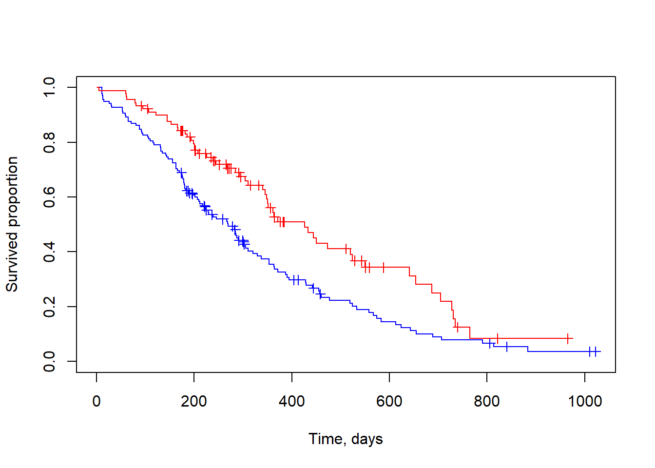
4.2.2. Cox model
Cox proportional hazards model, a.k.a. Cox model or Cox regression, is a statistical technique used in survival analysis. It models the time it takes for a certain event, like death, to occur as a function of predictor variables, without need to specify the form of the baseline hazard function. This allows for the estimation of the effect of the predictor variables on the hazard, or the event rate, at any given time.
Hazard function \(h(t)\) depends on basic hazard \(h_0(t)\) and variables \(x_1,..,x_n\):
\[h(t) = h_0(t) \times e^{\beta_1x_1+\beta_2x_2+...+\beta_nx_n} \] here \(\beta_i\) are fitted variables.
Hazard ratio (HR): \[HR = \frac{h_A(t)}{h_B(t)} = \exp{[\beta_1(x_{A1}-x_{B1}) + ... + \beta_n(x_{An}-x_{Bn})]}\] Working with log hazard ratio (LHR) makes life a bit easier. :)
\[LHR = \log({h_A(t)}) - \log({h_B(t)}) =
\beta_1(x_{A1}-x_{B1}) + ... + \beta_n(x_{An}-x_{Bn})\] Let’s
build Cox regression for lung data using a single variable
- sex
coxmod1 = coxph(sData ~ sex, data=lung)
summary(coxmod1)
## Call:
## coxph(formula = sData ~ sex, data = lung)
##
## n= 228, number of events= 165
##
## coef exp(coef) se(coef) z Pr(>|z|)
## sex -0.5310 0.5880 0.1672 -3.176 0.00149 **
## ---
## Signif. codes: 0 '***' 0.001 '**' 0.01 '*' 0.05 '.' 0.1 ' ' 1
##
## exp(coef) exp(-coef) lower .95 upper .95
## sex 0.588 1.701 0.4237 0.816
##
## Concordance= 0.579 (se = 0.021 )
## Likelihood ratio test= 10.63 on 1 df, p=0.001
## Wald test = 10.09 on 1 df, p=0.001
## Score (logrank) test = 10.33 on 1 df, p=0.001## build Cox regression model with 2 variables
mod2 = coxph(sData ~ sex + age, data=lung)
summary(mod2)## Call:
## coxph(formula = sData ~ sex + age, data = lung)
##
## n= 228, number of events= 165
##
## coef exp(coef) se(coef) z Pr(>|z|)
## sex -0.513219 0.598566 0.167458 -3.065 0.00218 **
## age 0.017045 1.017191 0.009223 1.848 0.06459 .
## ---
## Signif. codes: 0 '***' 0.001 '**' 0.01 '*' 0.05 '.' 0.1 ' ' 1
##
## exp(coef) exp(-coef) lower .95 upper .95
## sex 0.5986 1.6707 0.4311 0.8311
## age 1.0172 0.9831 0.9990 1.0357
##
## Concordance= 0.603 (se = 0.025 )
## Likelihood ratio test= 14.12 on 2 df, p=9e-04
## Wald test = 13.47 on 2 df, p=0.001
## Score (logrank) test = 13.72 on 2 df, p=0.001## build multivariable Cox regression model (can be problematic!)
mod3 = coxph(sData ~ ., data=lung[,-(1:3)])
summary(mod3)## Call:
## coxph(formula = sData ~ ., data = lung[, -(1:3)])
##
## n= 168, number of events= 121
## (60 observations deleted due to missingness)
##
## coef exp(coef) se(coef) z Pr(>|z|)
## age 1.065e-02 1.011e+00 1.161e-02 0.917 0.35906
## sex -5.509e-01 5.765e-01 2.008e-01 -2.743 0.00609 **
## ph.ecog 7.342e-01 2.084e+00 2.233e-01 3.288 0.00101 **
## ph.karno 2.246e-02 1.023e+00 1.124e-02 1.998 0.04574 *
## pat.karno -1.242e-02 9.877e-01 8.054e-03 -1.542 0.12316
## meal.cal 3.329e-05 1.000e+00 2.595e-04 0.128 0.89791
## wt.loss -1.433e-02 9.858e-01 7.771e-03 -1.844 0.06518 .
## ---
## Signif. codes: 0 '***' 0.001 '**' 0.01 '*' 0.05 '.' 0.1 ' ' 1
##
## exp(coef) exp(-coef) lower .95 upper .95
## age 1.0107 0.9894 0.9880 1.0340
## sex 0.5765 1.7347 0.3889 0.8545
## ph.ecog 2.0838 0.4799 1.3452 3.2277
## ph.karno 1.0227 0.9778 1.0004 1.0455
## pat.karno 0.9877 1.0125 0.9722 1.0034
## meal.cal 1.0000 1.0000 0.9995 1.0005
## wt.loss 0.9858 1.0144 0.9709 1.0009
##
## Concordance= 0.651 (se = 0.029 )
## Likelihood ratio test= 28.33 on 7 df, p=2e-04
## Wald test = 27.58 on 7 df, p=3e-04
## Score (logrank) test = 28.41 on 7 df, p=2e-04We cannot visualize directly Cox model with Kaplan-Meier. You have to use univariable model with categorization of the variable.
## Vizualize results of the Cox regression (univariable)
mod4 = coxph(sData ~ ph.ecog, data=lung)
summary(mod4)
## Call:
## coxph(formula = sData ~ ph.ecog, data = lung)
##
## n= 227, number of events= 164
## (1 observation deleted due to missingness)
##
## coef exp(coef) se(coef) z Pr(>|z|)
## ph.ecog 0.4759 1.6095 0.1134 4.198 2.69e-05 ***
## ---
## Signif. codes: 0 '***' 0.001 '**' 0.01 '*' 0.05 '.' 0.1 ' ' 1
##
## exp(coef) exp(-coef) lower .95 upper .95
## ph.ecog 1.61 0.6213 1.289 2.01
##
## Concordance= 0.604 (se = 0.024 )
## Likelihood ratio test= 17.57 on 1 df, p=3e-05
## Wald test = 17.62 on 1 df, p=3e-05
## Score (logrank) test = 17.89 on 1 df, p=2e-05fact = as.integer(lung$ph.ecog > median(lung$ph.ecog, na.rm = TRUE))
fact = factor(c("low","high")[fact+1],levels=c("low","high"))
fit.ph.ecog = survfit(sData ~ fact)
plot(fit.ph.ecog, col=c("blue","red"), mark.time=TRUE, xlab="Time, days", ylab="Survived", main="ph.ecog score low and high")
legend("topright",c("ph.ecog < median","ph.ecog > median"),col=c("blue","red"),lty=1)
4.2.3. Survival analysis in omics: combining variables
Now let’s take transcriptomics dataset from TCGA: melanoma (SKCM)
Download data:
library(survival)
download.file("http://edu.modas.lu/data/rda/SKCM.RData","SKCM.RData",mode="wb")
load("SKCM.RData")
str(Data)
Now, let’s work with the dataset.
str(Data)## List of 6
## $ ns : int 473
## $ nf : int 20531
## $ anno.file: chr "D:/Data/TCGA/TCGA.hg19.June2011.gaf"
## $ anno :'data.frame': 20531 obs. of 2 variables:
## ..$ gene : chr [1:20531] "?|100130426" "?|100133144" "?|100134869" "?|10357" ...
## ..$ location: chr [1:20531] "chr9:79791679-79792806:+" "chr15:82647286-82708202:+;chr15:83023773-83084727:+" "chr15:82647286-82707815:+;chr15:83023773-83084340:+" "chr20:56063450-56064083:-" ...
## $ meta :'data.frame': 473 obs. of 61 variables:
## ..$ data.files : chr [1:473] "unc.edu.00624286-41dd-476f-a63b-d2a5f484bb45.2250155.rsem.genes.results" "unc.edu.01c6644f-c721-4f5e-afbc-c220218941d8.2557685.rsem.genes.results" "unc.edu.020f448b-0242-4ff7-912a-4598d0b49055.1211973.rsem.genes.results" "unc.edu.02486980-eb4f-4930-ba27-356e346929b6.1677015.rsem.genes.results" ...
## ..$ barcode : chr [1:473] "TCGA-GN-A4U7-06A-21R-A32P-07" "TCGA-W3-AA1V-06B-11R-A40A-07" "TCGA-FS-A1Z0-06A-11R-A18T-07" "TCGA-D9-A3Z1-06A-11R-A239-07" ...
## ..$ disease : chr [1:473] "SKCM" "SKCM" "SKCM" "SKCM" ...
## ..$ sample_type : chr [1:473] "TM" "TM" "TM" "TM" ...
## ..$ center : chr [1:473] "UNC-LCCC" "UNC-LCCC" "UNC-LCCC" "UNC-LCCC" ...
## ..$ platform : chr [1:473] "ILLUMINA" "ILLUMINA" "ILLUMINA" "ILLUMINA" ...
## ..$ aliquot_id : chr [1:473] "00624286-41dd-476f-a63b-d2a5f484bb45" "01c6644f-c721-4f5e-afbc-c220218941d8" "020f448b-0242-4ff7-912a-4598d0b49055" "02486980-eb4f-4930-ba27-356e346929b6" ...
## ..$ participant_id : chr [1:473] "088c296e-8e13-4dc8-8a99-b27f4b27f95e" "9817ec15-605a-40db-b848-2199e5ccbb7b" "6a1966c3-7f01-4304-b4a1-c4ef683b179a" "4f7e7a0e-4aa2-4b6a-936f-6429c7d6a2a7" ...
## ..$ sample_type_name : Factor w/ 4 levels "Additional Metastatic",..: 2 2 2 2 2 2 3 2 2 2 ...
## ..$ bcr_patient_uuid : chr [1:473] "088C296E-8E13-4DC8-8A99-B27F4B27F95E" "9817EC15-605A-40DB-B848-2199E5CCBB7B" "6A1966C3-7F01-4304-B4A1-C4EF683B179A" "4F7E7A0E-4AA2-4B6A-936F-6429C7D6A2A7" ...
## ..$ bcr_patient_barcode : chr [1:473] "TCGA-GN-A4U7" "TCGA-W3-AA1V" "TCGA-FS-A1Z0" "TCGA-D9-A3Z1" ...
## ..$ form_completion_date : chr [1:473] "2013-8-19" "2014-7-17" "2012-11-12" "2012-7-24" ...
## ..$ prospective_collection : Factor w/ 2 levels "NO","YES": 1 1 1 2 1 2 2 1 1 1 ...
## ..$ retrospective_collection : Factor w/ 2 levels "NO","YES": 2 2 2 1 2 1 1 2 2 2 ...
## ..$ birth_days_to : num [1:473] -20458 -23314 -11815 -24192 -16736 ...
## ..$ gender : Factor w/ 2 levels "FEMALE","MALE": 1 2 1 2 2 1 2 2 1 2 ...
## ..$ height_cm_at_diagnosis : num [1:473] 161 180 NA 180 NA 160 173 182 NA NA ...
## ..$ weight_kg_at_diagnosis : num [1:473] 48 91 NA 80 NA 96 94 108 105 NA ...
## ..$ race : Factor w/ 3 levels "ASIAN","BLACK OR AFRICAN AMERICAN",..: 3 3 3 3 3 3 3 3 3 3 ...
## ..$ ethnicity : Factor w/ 2 levels "HISPANIC OR LATINO",..: 2 2 2 2 2 2 2 2 2 2 ...
## ..$ history_other_malignancy : Factor w/ 2 levels "No","Yes": 1 1 1 1 1 1 1 1 1 1 ...
## ..$ history_neoadjuvant_treatment : Factor w/ 2 levels "No","Yes": 1 1 1 1 1 1 1 2 1 1 ...
## ..$ tumor_status : Factor w/ 2 levels "TUMOR FREE","WITH TUMOR": 2 2 2 1 1 NA 1 2 1 2 ...
## ..$ vital_status : Factor w/ 2 levels "Alive","Dead": 1 2 2 1 1 1 1 2 1 2 ...
## ..$ last_contact_days_to : num [1:473] 266 NA NA 345 690 ...
## ..$ death_days_to : num [1:473] NA 1280 6164 NA NA ...
## ..$ primary_melanoma_known_dx : Factor w/ 2 levels "NO","YES": 2 2 2 2 1 2 2 2 2 2 ...
## ..$ primary_multiple_at_dx : Factor w/ 2 levels "NO","YES": 1 1 1 1 NA 1 NA 1 1 1 ...
## ..$ primary_at_dx_count : Factor w/ 4 levels "0","1","2","3": 2 NA 2 2 NA 2 NA NA 2 NA ...
## ..$ breslow_thickness_at_diagnosis : num [1:473] 1.39 1.3 0.95 1.7 NA 4 10 4.6 2.51 29 ...
## ..$ clark_level_at_diagnosis : Factor w/ 5 levels "I","II","III",..: 4 4 3 4 NA NA 3 NA 4 5 ...
## ..$ primary_melanoma_tumor_ulceration : Factor w/ 2 levels "NO","YES": 1 1 1 NA NA 2 2 2 1 1 ...
## ..$ primary_melanoma_mitotic_rate : num [1:473] 8 NA NA NA NA NA NA 15 9 9 ...
## ..$ initial_pathologic_dx_year : num [1:473] 2011 1994 1990 2011 2012 ...
## ..$ age_at_diagnosis : num [1:473] 56 63 32 66 45 74 53 64 29 57 ...
## ..$ ajcc_staging_edition : Factor w/ 7 levels "1st","2nd","3rd",..: 7 4 3 7 7 7 7 7 5 6 ...
## ..$ ajcc_tumor_pathologic_pt : Factor w/ 15 levels "T0","T1","T1a",..: 7 8 3 6 15 10 13 13 9 12 ...
## ..$ ajcc_nodes_pathologic_pn : Factor w/ 10 levels "N0","N1","N1a",..: 9 1 1 9 4 2 10 1 1 1 ...
## ..$ ajcc_metastasis_pathologic_pm : Factor w/ 5 levels "M0","M1","M1a",..: 1 1 1 1 1 1 1 1 1 1 ...
## ..$ ajcc_pathologic_tumor_stage : Factor w/ 14 levels "I/II NOS","Stage 0",..: 13 6 4 13 12 12 9 9 6 8 ...
## ..$ submitted_tumor_dx_days_to : num [1:473] 148 946 5440 223 26 ...
## ..$ submitted_tumor_site : Factor w/ 7 levels "Extremities",..: 1 5 1 NA NA 4 6 1 1 6 ...
## ..$ submitted_tumor_site.1 : Factor w/ 4 levels "Distant Metastasis",..: 4 4 1 4 4 4 2 4 4 4 ...
## ..$ metastatic_tumor_site : Factor w/ 52 levels "abdomen","Abdominal wall",..: NA NA 42 NA NA NA NA NA NA NA ...
## ..$ primary_melanoma_skin_type : Factor w/ 1 level "Non-glabrous skin": 1 1 1 NA 1 1 1 1 NA 1 ...
## ..$ radiation_treatment_adjuvant : Factor w/ 2 levels "NO","YES": 1 1 1 1 2 1 1 1 1 1 ...
## ..$ pharmaceutical_tx_adjuvant : Factor w/ 2 levels "NO","YES": 1 2 1 1 1 NA 1 2 2 1 ...
## ..$ new_tumor_event_dx_indicator : Factor w/ 2 levels "NO","YES": 2 2 2 1 2 2 1 1 2 2 ...
## ..$ new_tumor_event_prior_to_bcr_tumor : Factor w/ 2 levels "NO","YES": 1 1 NA NA 1 1 NA NA 1 1 ...
## ..$ new_tumor_event_melanoma_count : Factor w/ 5 levels "1","1|1","1|2",..: 1 1 NA NA NA 1 1 NA 1 NA ...
## ..$ days_to_initial_pathologic_diagnosis: Factor w/ 1 level "0": 1 1 1 1 1 1 1 1 1 1 ...
## ..$ icd_10 : Factor w/ 48 levels "C07","C17.9",..: 47 45 20 45 45 46 16 48 45 14 ...
## ..$ icd_o_3_histology : Factor w/ 10 levels "8720/3","8721/3",..: 1 1 1 1 1 1 1 1 1 1 ...
## ..$ icd_o_3_site : Factor w/ 44 levels "C07.9","C17.9",..: 43 41 17 41 41 42 15 44 41 14 ...
## ..$ informed_consent_verified : Factor w/ 1 level "YES": 1 1 1 1 1 1 1 1 1 1 ...
## ..$ patient_id : chr [1:473] "A4U7" "AA1V" "A1Z0" "A3Z1" ...
## ..$ tissue_source_site : Factor w/ 25 levels "3N","BF","D3",..: 13 20 10 4 21 6 6 3 9 7 ...
## ..$ fact_age : Factor w/ 4 levels "age1","age2",..: 2 3 1 3 1 4 2 3 1 2 ...
## ..$ fact_surv : Factor w/ 3 levels "good","poor",..: 3 1 1 3 3 3 3 2 1 2 ...
## ..$ surv_event : int [1:473] 0 1 1 0 0 0 0 1 0 1 ...
## ..$ surv_time : num [1:473] 266 1280 6164 345 690 ...
## $ x : num [1:20531, 1:473] 0 1.8 1.84 6.42 10.89 ...
## ..- attr(*, "dimnames")=List of 2
## .. ..$ : chr [1:20531] "?|100130426" "?|100133144" "?|100134869" "?|10357" ...
## .. ..$ : chr [1:473] "TCGA-GN-A4U7-06A-21R-A32P-07" "TCGA-W3-AA1V-06B-11R-A40A-07" "TCGA-FS-A1Z0-06A-11R-A18T-07" "TCGA-D9-A3Z1-06A-11R-A239-07" ...Sur = Surv(time = Data$meta$surv_time, event = Data$meta$surv_event)
## keep expressed genes
ikeep = apply(Data$x,1,max) > 5
X = Data$x[ikeep,]
## build container and Cox regression for each gene
Res = data.frame(Gene = rownames(X), LHR=NA, PV = 1, FDR=1)
rownames(Res) = rownames(X)
ig=1
for (ig in 1:nrow(X)){
mod = coxph(Sur ~ X[ig,])
Res$LHR[ig] = summary(mod)$coefficients[,"coef"]
Res$PV[ig] = summary(mod)$sctest["pvalue"]
## write message every 1000 genes
if(ig%%1000 == 0){
print(ig)
flush.console()
}
}## [1] 1000
## [1] 2000
## [1] 3000## Warning in coxph.fit(X, Y, istrat, offset, init, control, weights = weights, :
## Loglik converged before variable 1 ; coefficient may be infinite.## [1] 4000
## [1] 5000## Warning in coxph.fit(X, Y, istrat, offset, init, control, weights = weights, :
## Loglik converged before variable 1 ; coefficient may be infinite.## [1] 6000
## [1] 7000## Warning in coxph.fit(X, Y, istrat, offset, init, control, weights = weights, :
## Loglik converged before variable 1 ; coefficient may be infinite.## [1] 8000
## [1] 9000
## [1] 10000
## [1] 11000
## [1] 12000## Warning in coxph.fit(X, Y, istrat, offset, init, control, weights = weights, :
## Loglik converged before variable 1 ; coefficient may be infinite.## [1] 13000
## [1] 14000
## [1] 15000## Warning in coxph.fit(X, Y, istrat, offset, init, control, weights = weights, :
## Loglik converged before variable 1 ; coefficient may be infinite.## [1] 16000
## [1] 17000
## [1] 18000Res$FDR = p.adjust(Res$PV,method="fdr")
str(Res)## 'data.frame': 18159 obs. of 4 variables:
## $ Gene: chr "?|100133144" "?|100134869" "?|10357" "?|10431" ...
## $ LHR : num -0.125 -0.128 0.0764 0.2797 -0.1135 ...
## $ PV : num 0.0519 0.0825 0.557 0.0704 0.1773 ...
## $ FDR : num 0.248 0.312 0.788 0.288 0.452 ...isig = Res$FDR<0.01
Res[isig,-1]## LHR PV FDR
## APOBEC3G|60489 -0.2047082 1.212530e-05 0.007435642
## B2M|567 -0.2726906 1.583459e-05 0.007999758
## BTN3A1|11119 -0.3029528 4.345391e-05 0.009856823
## C17orf75|64149 -0.3256536 3.638734e-05 0.009856823
## C1RL|51279 -0.2781420 1.580211e-06 0.003586881
## C5orf58|133874 -0.1955139 4.500883e-05 0.009856823
## C6orf10|10665 0.2389909 3.401933e-05 0.009849785
## CBLN2|147381 0.1404172 8.623512e-06 0.006524765
## CCL8|6355 -0.1755091 2.149351e-06 0.003903006
## CLEC2B|9976 -0.2682245 3.857981e-06 0.005288683
## CLEC6A|93978 -0.3102829 4.229019e-05 0.009856823
## CLEC7A|64581 -0.1789562 4.403990e-05 0.009856823
## CSGALNACT1|55790 -0.2163559 3.014911e-05 0.009279284
## CTBS|1486 -0.4237893 3.506018e-05 0.009849785
## CXCL10|3627 -0.1184127 3.475051e-05 0.009849785
## CXCL11|6373 -0.1271245 3.768840e-05 0.009856823
## DDX60L|91351 -0.2741668 1.698725e-05 0.008008019
## DDX60|55601 -0.2638947 1.070490e-06 0.003586881
## DTX3L|151636 -0.2916345 4.606690e-05 0.009856823
## ELSPBP1|64100 0.1878215 1.265218e-06 0.003586881
## FAM105A|54491 -0.1949298 2.529268e-05 0.009253244
## FAM122C|159091 -0.4943014 2.598796e-05 0.009253244
## FAM83C|128876 0.1552354 1.990499e-05 0.008815967
## FAM96A|84191 -0.5566587 3.202989e-05 0.009693845
## FCGR2A|2212 -0.2475779 2.105254e-05 0.008890537
## FCGR2C|9103 -0.1971861 3.757665e-05 0.009856823
## GABRA5|2558 0.1415025 1.147964e-06 0.003586881
## GATAD2A|54815 0.7332271 7.151997e-06 0.006317774
## GBP2|2634 -0.2203771 4.662014e-07 0.003586881
## GBP4|115361 -0.1446505 1.719879e-05 0.008008019
## GBP5|115362 -0.1204195 3.842002e-05 0.009856823
## GCNT1|2650 -0.2171306 1.124155e-05 0.007435642
## GIMAP2|26157 -0.2431658 2.015502e-06 0.003903006
## GORAB|92344 -0.3538969 2.376937e-05 0.009253244
## GPR171|29909 -0.1584386 2.890531e-05 0.009276137
## GRWD1|83743 0.5961874 3.877483e-05 0.009856823
## HAPLN3|145864 -0.2994643 1.480725e-06 0.003586881
## HCG26|352961 -0.1865897 1.576804e-05 0.007999758
## HCP5|10866 -0.1628275 1.585942e-05 0.007999758
## HN1L|90861 0.7600924 2.433009e-05 0.009253244
## HSPA7|3311 -0.2013804 2.925736e-06 0.004644880
## IFIH1|64135 -0.2500093 6.453365e-06 0.006317774
## IFITM1|8519 -0.1904017 4.212032e-05 0.009856823
## KCTD18|130535 -0.5113143 2.743567e-05 0.009276137
## KIR3DX1|90011 -0.5735384 2.842172e-05 0.009276137
## KLRD1|3824 -0.1516582 3.953009e-05 0.009856823
## LHB|3972 0.1996116 4.312092e-05 0.009856823
## LOC100128675|100128675 -0.1196206 1.309747e-05 0.007435642
## LOC220930|220930 -0.2266815 6.366743e-06 0.006317774
## LOC400759|400759 -0.1428890 4.091954e-05 0.009856823
## MANEA|79694 -0.2875416 2.723321e-05 0.009276137
## MIR155HG|114614 -0.1809546 2.911723e-05 0.009276137
## MRPS2|51116 0.4226844 3.441944e-05 0.009849785
## N4BP2L1|90634 -0.2682710 4.309698e-06 0.005288683
## NCCRP1|342897 0.1404060 6.859614e-06 0.006317774
## NEK7|140609 -0.3362469 2.557320e-05 0.009253244
## NEURL3|93082 -0.2096818 4.618223e-05 0.009856823
## NMI|9111 -0.2723000 2.060890e-05 0.008890537
## NOLC1|9221 0.5868476 4.006145e-05 0.009856823
## NXT2|55916 -0.3360888 9.857932e-06 0.007160408
## PARP12|64761 -0.2461374 1.268991e-05 0.007435642
## PARP14|54625 -0.2910446 1.825817e-05 0.008288755
## PARP9|83666 -0.2819776 1.373288e-05 0.007556831
## PCMTD1|115294 -0.3764190 2.464025e-05 0.009253244
## PIK3R2|5296 0.5573897 4.863629e-05 0.009983333
## PRKAR2B|5577 -0.2425505 1.651434e-05 0.008008019
## PTPN22|26191 -0.1612571 3.525723e-05 0.009849785
## PYHIN1|149628 -0.1383337 3.010298e-05 0.009279284
## RAP1A|5906 -0.4739783 2.759056e-05 0.009276137
## RARRES3|5920 -0.1686688 7.206203e-06 0.006317774
## RBM43|375287 -0.2988122 3.069473e-06 0.004644880
## RWDD2A|112611 -0.4363977 4.722417e-05 0.009856823
## SAMD9L|219285 -0.1834091 4.630687e-05 0.009856823
## SATB1|6304 -0.2096225 4.927852e-07 0.003586881
## SLC5A3|6526 -0.2673013 4.368646e-06 0.005288683
## SLFN12|55106 -0.2538958 1.544767e-06 0.003586881
## SLFN13|146857 -0.2027953 4.892982e-05 0.009983333
## SRGN|5552 -0.2388324 4.275872e-05 0.009856823
## STAT1|6772 -0.2609808 2.335639e-05 0.009253244
## TLR2|7097 -0.2131466 4.540749e-05 0.009856823
## TRIM22|10346 -0.2107059 1.310317e-05 0.007435642
## TRIM29|23650 0.1129338 8.103264e-06 0.006397703
## TTC39C|125488 -0.2378104 7.654113e-06 0.006317774
## UBA7|7318 -0.2302119 7.555765e-06 0.006317774
## UBE2L6|9246 -0.2874326 1.098596e-05 0.007435642
## XRN1|54464 -0.3427680 2.461182e-05 0.009253244
## ZC3H6|376940 -0.4257080 1.205231e-05 0.007435642
## ZNF25|219749 -0.3241123 4.028288e-05 0.009856823
## ZNF831|128611 -0.1432127 4.691070e-05 0.009856823## make a KM plot
## gene -> factor
ibest = which.min(Res$FDR)
fgene = c("low","high")[1+as.integer(X[ibest,]>median(X[ibest,]))]
fgene = factor(fgene,levels=c("low","high"))
plot(survfit(Sur ~ fgene),col=c(4,2),lwd=c(2,1,1), conf.int = TRUE, mark.time=TRUE,
main=sprintf("Best gene %s, pval = %.2e",Res[ibest,"Gene"],Res[ibest,"PV"]))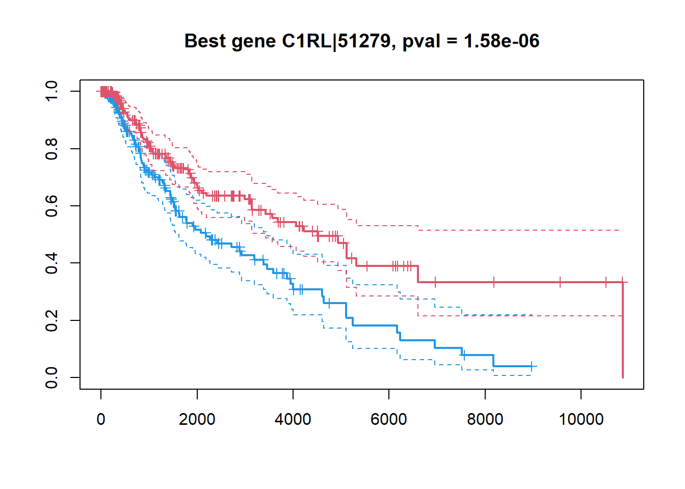
## lets combine genes
score = double(ncol(X))
ip=1
for (ip in 1:ncol(X)){
    score[ip] = sum(Res$LHR[isig] * X[isig,ip])
}

mod = coxph(Sur~score)
summary(mod)
## Call:
## coxph(formula = Sur ~ score)
##
## n= 463, number of events= 154
## (10 observations deleted due to missingness)
##
## coef exp(coef) se(coef) z Pr(>|z|)
## score 0.031922 1.032437 0.004321 7.389 1.48e-13 ***
## ---
## Signif. codes: 0 '***' 0.001 '**' 0.01 '*' 0.05 '.' 0.1 ' ' 1
##
## exp(coef) exp(-coef) lower .95 upper .95
## score 1.032 0.9686 1.024 1.041
##
## Concordance= 0.682 (se = 0.024 )
## Likelihood ratio test= 51.05 on 1 df, p=9e-13
## Wald test = 54.59 on 1 df, p=1e-13
## Score (logrank) test = 56.33 on 1 df, p=6e-14## make a KM plot
## score -> factor
fscore = c("low","high")[1+as.integer(score>median(score))]
fscore = factor(fscore,levels=c("low","high"))
plot(survfit(Sur ~ fscore),col=c(4,2),lwd=c(2,1,1), conf.int = TRUE, mark.time=TRUE,
main=sprintf("Combined score, pval = %.2e", summary(mod)$sctest["pvalue"]))
4.3. DIMENSIONALITY REDUCTION
4.3.1. Overview of dimensionality reduction methods

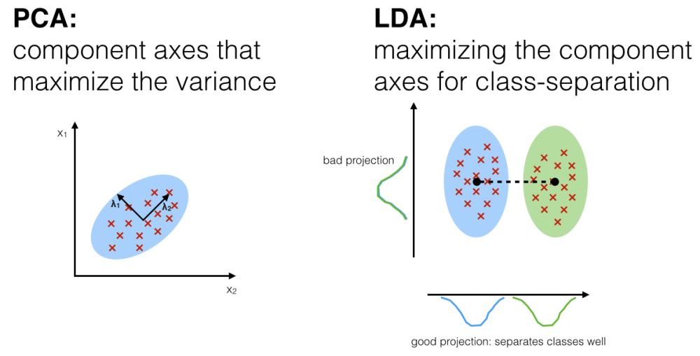
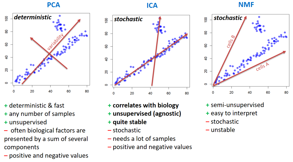
PCA (principal component analysis) - rotation of the coordinate system in multidimensional space in the way to capture main variability in the data.
ICA (independent component analysis) - matrix factorization method that identifies statistically independent signals and their weights.
NMF (non-negative matrix factorization) - matrix factorization method that presents data as a matrix product of two non-negative matrices.
LDA (linear discriminant analysis) - identify new coordinate system, maximizing difference between objects belonging to predefined groups.
MDS (multi-dimensional scaling) - method that tries to preserve distances between objects in the low-dimension space.
VAE (variational autoencoder) - artificial neural network with a “bottle-neck”, allowing smooth projection of data to low-dimensional space.
t-SNE (t-distributed stochastic neighbor embedding) - an iterative approach, similar to MDS, but considering only close objects. Thus, similar objects must be close in the new (reduced) space, while distant objects are not influencing the results.
UMAP (uniform manifold approximation and projection) - modern method, similar to t-SNE, but more stable and with preservation of some information about distant groups (preserving the topology of the data).
Let’s consider some nice resources online:
Principal Component Analysis Explained Visually by Victor Powell
Understanding UMAP by Andy Coenen and Adam Pearce
Dimensionality Reduction for Data Visualization: PCA vs TSNE vs UMAP vs LDA by Sivakar Sivarajah
4.3.2. PCA - Principle Component Analysis
PCA of samples in the space of features (genes/proteins)
Simplest way to do PCA in R is to use default prcomp()
function. It takes a matrix with samples in rows and features in
columns.
- If you assume that absolute values of features is not important
(only relative variability) - use
scale=TRUE.
## load the script from Internet
source("http://r.modas.lu/readAMD.r")

## read mRNA data (automatic annotation of samples)
mRNA = readAMD("http://edu.modas.lu/data/txt/mrna_ifng.amd.txt",
               stringsAsFactors = TRUE,
               index.column="GeneSymbol",
               sum.func="mean")
## [1] "Repeated feature IDs => data are summarized (mean) by row"
## [1] "Performing summarization: 33297 rows -> 20141 rows by <mean>"
##
|
| | 0%
|
| | 1%
|
|= | 1%
|
|= | 2%
|
|== | 2%
|
|== | 3%
|
|== | 4%
|
|=== | 4%
|
|=== | 5%
|
|==== | 5%
|
|==== | 6%
|
|===== | 6%
|
|===== | 7%
|
|===== | 8%
|
|====== | 8%
|
|====== | 9%
|
|======= | 9%
|
|======= | 10%
|
|======= | 11%
|
|======== | 11%
|
|======== | 12%
|
|========= | 12%
|
|========= | 13%
|
|========= | 14%
|
|========== | 14%
|
|========== | 15%
|
|=========== | 15%
|
|=========== | 16%
|
|============ | 16%
|
|============ | 17%
|
|============ | 18%
|
|============= | 18%
|
|============= | 19%
|
|============== | 19%
|
|============== | 20%
|
|============== | 21%
|
|=============== | 21%
|
|=============== | 22%
|
|================ | 22%
|
|================ | 23%
|
|================ | 24%
|
|================= | 24%
|
|================= | 25%
|
|================== | 25%
|
|================== | 26%
|
|=================== | 26%
|
|=================== | 27%
|
|=================== | 28%
|
|==================== | 28%
|
|==================== | 29%
|
|===================== | 29%
|
|===================== | 30%
|
|===================== | 31%
|
|====================== | 31%
|
|====================== | 32%
|
|======================= | 32%
|
|======================= | 33%
|
|======================= | 34%
|
|======================== | 34%
|
|======================== | 35%
|
|========================= | 35%
|
|========================= | 36%
|
|========================== | 36%
|
|========================== | 37%
|
|========================== | 38%
|
|=========================== | 38%
|
|=========================== | 39%
|
|============================ | 39%
|
|============================ | 40%
|
|============================ | 41%
|
|============================= | 41%
|
|============================= | 42%
|
|============================== | 42%
|
|============================== | 43%
|
|============================== | 44%
|
|=============================== | 44%
|
|=============================== | 45%
|
|================================ | 45%
|
|================================ | 46%
|
|================================= | 46%
|
|================================= | 47%
|
|================================= | 48%
|
|================================== | 48%
|
|================================== | 49%
|
|=================================== | 49%
|
|=================================== | 50%
|
|=================================== | 51%
|
|==================================== | 51%
|
|==================================== | 52%
|
|===================================== | 52%
|
|===================================== | 53%
|
|===================================== | 54%
|
|====================================== | 54%
|
|====================================== | 55%
|
|======================================= | 55%
|
|======================================= | 56%
|
|======================================== | 56%
|
|======================================== | 57%
|
|======================================== | 58%
|
|========================================= | 58%
|
|========================================= | 59%
|
|========================================== | 59%
|
|========================================== | 60%
|
|========================================== | 61%
|
|=========================================== | 61%
|
|=========================================== | 62%
|
|============================================ | 62%
|
|============================================ | 63%
|
|============================================ | 64%
|
|============================================= | 64%
|
|============================================= | 65%
|
|============================================== | 65%
|
|============================================== | 66%
|
|=============================================== | 66%
|
|=============================================== | 67%
|
|=============================================== | 68%
|
|================================================ | 68%
|
|================================================ | 69%
|
|================================================= | 69%
|
|================================================= | 70%
|
|================================================= | 71%
|
|================================================== | 71%
|
|================================================== | 72%
|
|=================================================== | 72%
|
|=================================================== | 73%
|
|=================================================== | 74%
|
|==================================================== | 74%
|
|==================================================== | 75%
|
|===================================================== | 75%
|
|===================================================== | 76%
|
|====================================================== | 76%
|
|====================================================== | 77%
|
|====================================================== | 78%
|
|======================================================= | 78%
|
|======================================================= | 79%
|
|======================================================== | 79%
|
|======================================================== | 80%
|
|======================================================== | 81%
|
|========================================================= | 81%
|
|========================================================= | 82%
|
|========================================================== | 82%
|
|========================================================== | 83%
|
|========================================================== | 84%
|
|=========================================================== | 84%
|
|=========================================================== | 85%
|
|============================================================ | 85%
|
|============================================================ | 86%
|
|============================================================= | 86%
|
|============================================================= | 87%
|
|============================================================= | 88%
|
|============================================================== | 88%
|
|============================================================== | 89%
|
|=============================================================== | 89%
|
|=============================================================== | 90%
|
|=============================================================== | 91%
|
|================================================================ | 91%
|
|================================================================ | 92%
|
|================================================================= | 92%
|
|================================================================= | 93%
|
|================================================================= | 94%
|
|================================================================== | 94%
|
|================================================================== | 95%
|
|=================================================================== | 95%
|
|=================================================================== | 96%
|
|==================================================================== | 96%
|
|==================================================================== | 97%
|
|==================================================================== | 98%
|
|===================================================================== | 98%
|
|===================================================================== | 99%
|
|======================================================================| 99%
|
|======================================================================| 100%[1] "done in"
## Time difference of 1.273681 secsstr(mRNA)## List of 5
## $ ncol: int 17
## $ nrow: int 20141
## $ anno:'data.frame': 20141 obs. of 8 variables:
## ..$ GeneSymbol : chr [1:20141] "" "A1BG" "A1CF" "A2BP1" ...
## ..$ ID : chr [1:20141] "7892501,7892502,7892503,7892504,7892505,7892506,7892507,7892508,7892509,7892510,7892511,7892512,7892513,7892514"| __truncated__ "8039748" "7933640" "7993083,7993110" ...
## ..$ gene_assignment: chr [1:20141] "---," "NM_130786 // A1BG // alpha-1-B glycoprotein // 19q13.4 // 1 /// NM_198458 // ZNF497 // zinc finger protein 497 "| __truncated__ "NM_138933 // A1CF // APOBEC1 complementation factor // 10q11.23 // 29974 /// NM_014576 // A1CF // APOBEC1 compl"| __truncated__ "NM_018723 // A2BP1 // ataxin 2-binding protein 1 // 16p13.3 // 54715 /// NM_145893 // A2BP1 // ataxin 2-binding"| __truncated__ ...
## ..$ RefSeq : chr [1:20141] "---," "NM_130786" "NM_138933" "NM_018723,ENST00000432184" ...
## ..$ seqname : chr [1:20141] "---,chr1,chr10,,chr11,chr12,chr13,chrUn_gl000212,chr14,chr15,chr16,chr17,chr17_gl000205_random,chr18,chr19,chr2"| __truncated__ "chr19" "chr10" "chr16" ...
## ..$ start : chr [1:20141] " 0, 53049, 63015, 564951, 566062, 568844, 1102484, 1103243, 1104373, 2316811, 6600914, "| __truncated__ " 58856544" " 52566314" " 6069132, 6753884" ...
## ..$ stop : chr [1:20141] " 0, 54936, 63887, 565019, 566129, 568913, 1102578, 1103332, 1104471, 2319922, 6600994, "| __truncated__ " 58867591" " 52645435" " 7763340, 6755559" ...
## ..$ strand : chr [1:20141] "---,+,-," "-" "-" "+" ...
## $ meta:'data.frame': 17 obs. of 3 variables:
## ..$ time : Factor w/ 7 levels "T00","T03","T12",..: 1 1 2 2 3 3 4 4 4 5 ...
## ..$ treatment: Factor w/ 3 levels "IFNg","IFNg_JII",..: 3 3 1 1 1 1 1 1 1 1 ...
## ..$ replicate: Factor w/ 3 levels "r1","r2","r3": 1 2 1 2 1 2 1 2 3 1 ...
## $ X : num [1:20141, 1:17] 6.6 6.15 5.1 4.64 5.78 ...
## ..- attr(*, "dimnames")=List of 2
## .. ..$ : chr [1:20141] "" "A1BG" "A1CF" "A2BP1" ...
## .. ..$ : chr [1:17] "T00.1" "T00.2" "T03.1" "T03.2" ...PC = prcomp(t(mRNA$X),scale=TRUE)
str(PC)## List of 5
## $ sdev : num [1:17] 83.4 55.3 48.1 42 36 ...
## $ rotation: num [1:20141, 1:17] 0.001125 0.000754 0.006407 0.008881 0.009878 ...
## ..- attr(*, "dimnames")=List of 2
## .. ..$ : chr [1:20141] "" "A1BG" "A1CF" "A2BP1" ...
## .. ..$ : chr [1:17] "PC1" "PC2" "PC3" "PC4" ...
## $ center : Named num [1:20141] 6.6 6.25 5.1 4.64 5.92 ...
## ..- attr(*, "names")= chr [1:20141] "" "A1BG" "A1CF" "A2BP1" ...
## $ scale : Named num [1:20141] 0.0233 0.1059 0.1061 0.0862 0.2095 ...
## ..- attr(*, "names")= chr [1:20141] "" "A1BG" "A1CF" "A2BP1" ...
## $ x : num [1:17, 1:17] -84.9 -104.8 -69.3 -81.6 -70 ...
## ..- attr(*, "dimnames")=List of 2
## .. ..$ : chr [1:17] "T00.1" "T00.2" "T03.1" "T03.2" ...
## .. ..$ : chr [1:17] "PC1" "PC2" "PC3" "PC4" ...
## - attr(*, "class")= chr "prcomp"plot(PC$x[,"PC1"],PC$x[,"PC2"],col=as.integer(mRNA$meta$time),pch=19,cex=2,
main="PCA (scaled gene expression)")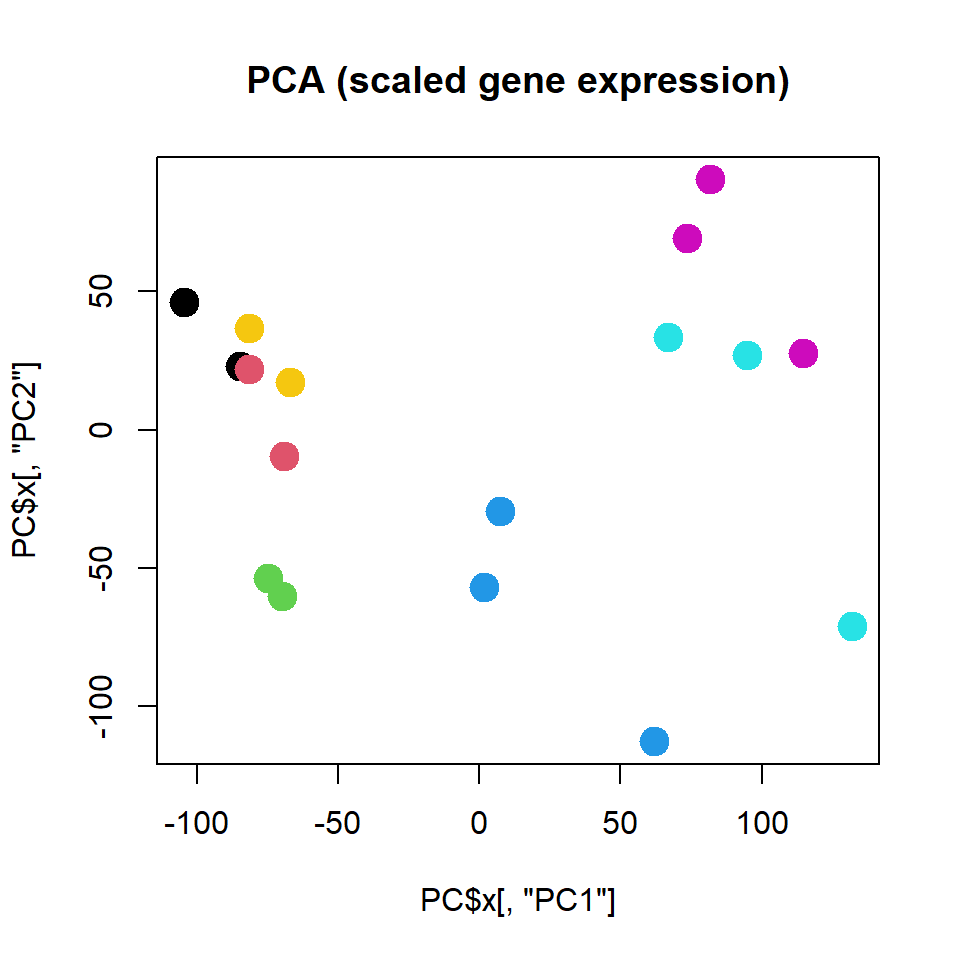
Alternatively you could use my warp-up function
plotPCA(). Let’s try it with and without gene scaling
source("http://sablab.net/scripts/plotPCA.r")
par(mfcol=c(1,2))
plotPCA(mRNA$X,col=as.integer(mRNA$meta$time),cex.names=1,cex=2,
        main="PCA (gene scaling)")
plotPCA(mRNA$X,col=as.integer(mRNA$meta$time),cex.names=1,cex=2, scale=FALSE,
        main="PCA (no scaling)")
Variability captured by each component can be calculated and visualized as a scree plot manualy:
## calculate percentage of variability
PC$pvar = (PC$sdev^2)/sum(PC$sdev^2)
names(PC$pvar) = colnames(PC$x)

## draw scree plot
barplot(PC$pvar[1:10],ylim = c(0,0.4), col="skyblue",main="Explained Variability",cex.main=1, xlab="Components",ylab="Variability explained")

## add text
text(1.2 * (1:10)-0.5,PC$pvar[1:10],sprintf("%.3f",PC$pvar[1:10]),adj=c(0.5,-1))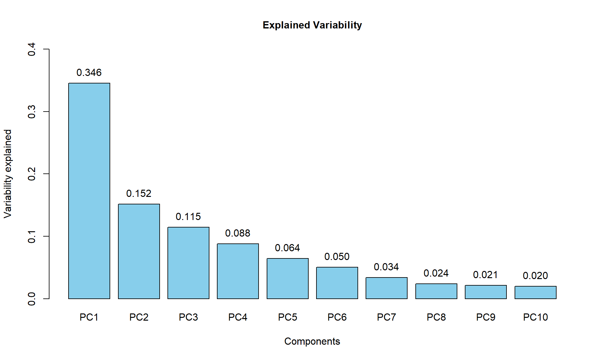
or using a package::function factoextra::fviz_eig() (try
it, if you wish).
factoextra::fviz_eig(PC, addlabels = TRUE, main="Explained Variability (fviz_eig)")
Another powerful package: PCAtools
## please install: PCAtools and ggalt

#install.packages("BiocManager")
#BiocManager::install("PCAtools")
#install.packages("ggalt")

library(PCAtools)
## Loading required package: ggrepel##
## Attaching package: 'PCAtools'## The following objects are masked from 'package:stats':
##
## biplot, screeplotp = pca(mRNA$X, removeVar = 0, metadata = mRNA$meta)## -- removing the lower 0% of variables based on variancebiplot(p, colby="time", title="Principal Component Analysis", legendPosition = "bottom", showLoadings = TRUE,encircle=TRUE)## Registered S3 methods overwritten by 'ggalt':
## method from
## grid.draw.absoluteGrob ggplot2
## grobHeight.absoluteGrob ggplot2
## grobWidth.absoluteGrob ggplot2
## grobX.absoluteGrob ggplot2
## grobY.absoluteGrob ggplot2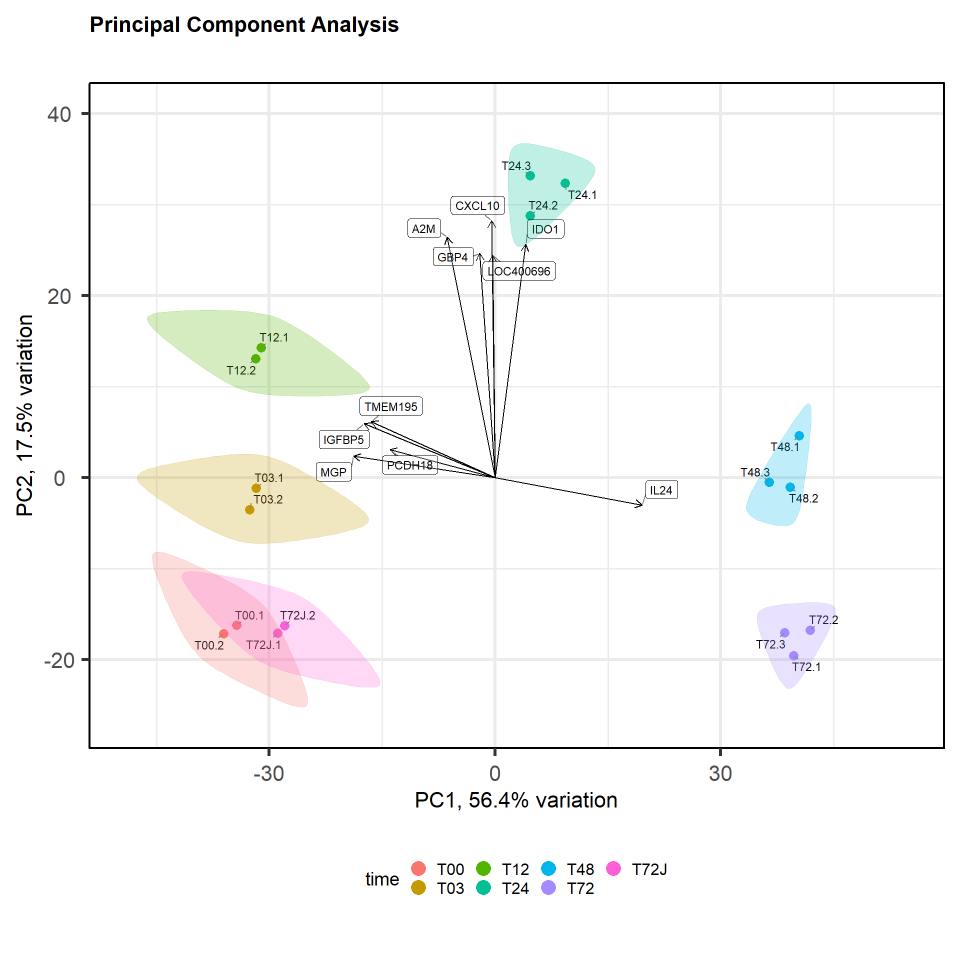
screeplot(p, axisLabSize = 8, titleLabSize = 22)
PCA of genes in the space of samples
We can also use PCA to see similarity between features. Let’s also highlight marker genes.
size = 0.5 + apply(mRNA$X,1,mean)/6

## Log intensities
plotPCA( t(mRNA$X),
         col="#00AA0022",
         cex=size,
         main = "PCA for genes (sample space)")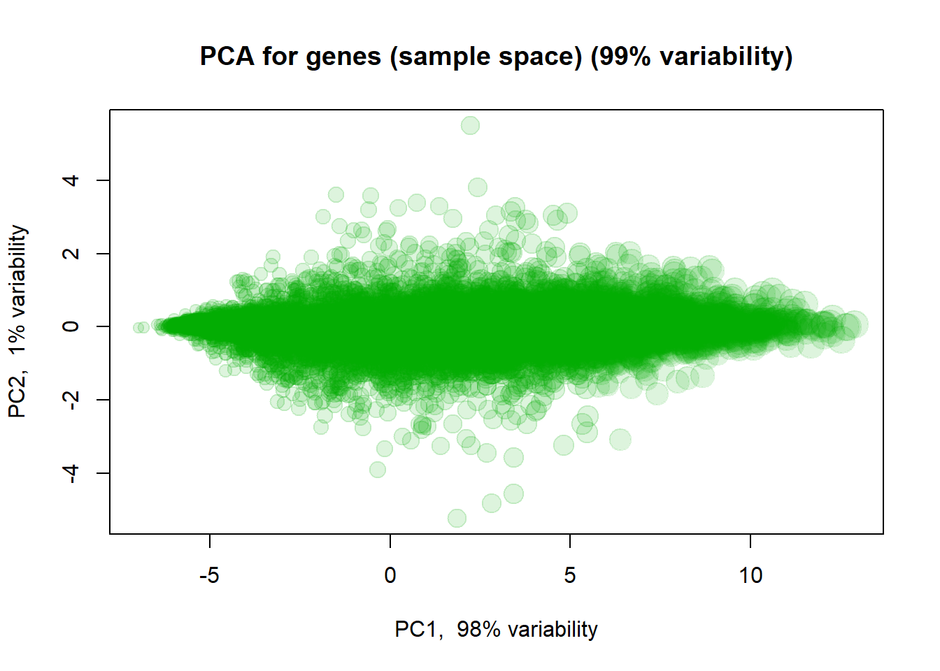
## you can check behaviour of with treatment "VEGFA","IRF1","SOX5This is not too informative, as 98% of variability is related to overall gene expression. Let’s normalize genes (each gene will have mean = 0, st.dev = 0 over samples).
## Let's scale expression
Z = mRNA$X
Z[,] = t(scale(t(Z)))

PC2 = prcomp(Z,scale=TRUE)
plotPCA(t(Z),pc = PC2,col="#00AA0011", cex=size, main = "Standardized expression (per gene)")

## select 3 genes and show them
genes = c(which.min(PC2$x[,1]),which.max(PC2$x[,1]),which.min(abs(PC2$x[,1]-2) * abs(PC2$x[,2]-1)))
text(PC2$x[genes,1],PC2$x[genes,2],names(genes),col=1,pch=19,font=2)
I selected here 3 genes for a detailed investigation:
## behaviour with treatment
par(mfcol=c(1,3))
boxplot(mRNA$X[genes[1],]~mRNA$meta$time, main = names(genes)[1], col = 1:nlevels(mRNA$meta$time))
boxplot(mRNA$X[genes[2],]~mRNA$meta$time, main = names(genes)[2], col = 1:nlevels(mRNA$meta$time))
boxplot(mRNA$X[genes[3],]~mRNA$meta$time, main = names(genes)[3], col = 1:nlevels(mRNA$meta$time))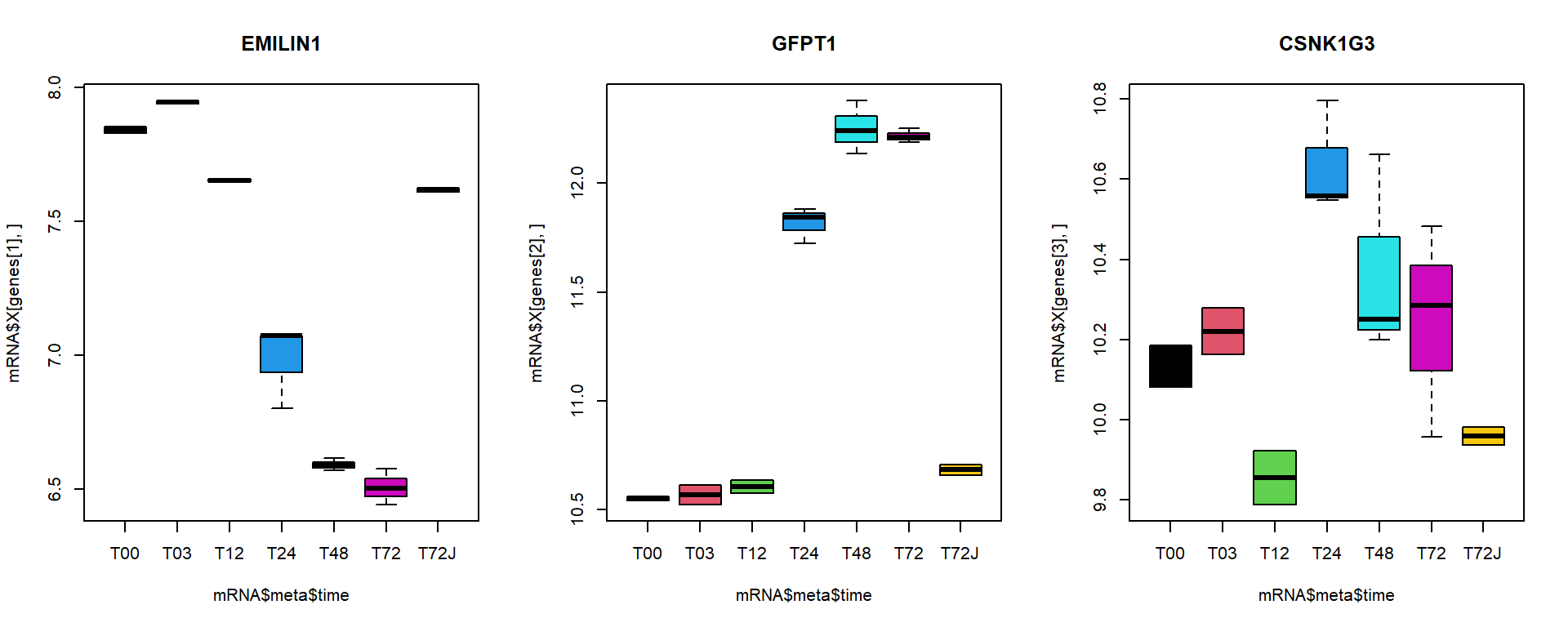
4.3.3. MDS
Classical MDS can be performed using cmdscale()
function
## calculate euclidean distances
d = dist(t(mRNA$X))

## fit distances in 2D space to distances in multidimensional space
MDS = cmdscale(d,k=2)
str(MDS)
## num [1:17, 1:2] -34.4 -36.1 -31.8 -32.6 -31.1 ...
## - attr(*, "dimnames")=List of 2
## ..$ : chr [1:17] "T00.1" "T00.2" "T03.1" "T03.2" ...
## ..$ : NULLplot(MDS[,1],MDS[,2],col=as.integer(mRNA$meta$time),pch=19, main="MDS plot",cex =2)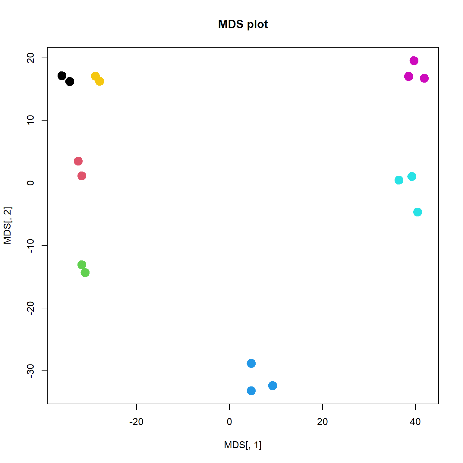
As you can see, it is very close to PCA results. But it requires much more computational power, when working with large number of objects. It may outperform PCA in a special case, when variance captured by 1st, 2nd and 3rd components is similar. Or when you need a special type of distance.
4.3.4. ICA
ICA, similar to PCA, but tries to extract statistically independent signals. This signals are correlated to biological processes more often than for PCA. But to see ICA power we need a lot of data. Here results will be similar to MDS.
source("http://r.modas.lu/LibICA.r")## [1] "----------------------------------------------------------------"
## [1] "libML: Machine learning library"
## [1] "Needed:"
## [1] "randomForest" "e1071"
## [1] "Absent:"
## character(0)
## [1] "----------------------------------------------------------------"
## [1] "consICA: Checking required packages and installing missing ones"
## [1] "Needed:"
## [1] "fastICA" "sm" "vioplot" "pheatmap" "gplots"
## [6] "foreach" "survival" "topGO" "org.Hs.eg.db" "org.Mm.eg.db"
## [11] "doSNOW"
## [1] "Absent:"
## character(0)IC = runICA(mRNA$X,ntry=100,ncomp=3,ncores=2)## Loading required package: fastICA## Loading required package: foreach## Loading required package: doSNOW## Loading required package: iterators## Loading required package: snow## *** Starting parallel calculation on 2 core(s)...
## *** System: windows
## *** 3 components, 100 runs, 20141 features, 17 samples.
## *** Start time: 2024-04-17 09:15:54.069265
## *** Done!
## *** End time: 2024-04-17 09:16:07.342023
## Time difference of 13.24992 secs
## Calculate ||X-SxM|| and r2 between component weights
## Correlate rows of S between tries
## Build consensus ICA
## Analyse stabilitypar(mfcol=c(1,3))
plot(IC$M[1,],IC$M[2,],pch=19,col=as.integer(mRNA$meta$time),cex=2,main="IC1-IC2")
plot(IC$M[1,],IC$M[3,],pch=19,col=as.integer(mRNA$meta$time),cex=2,main="IC1-IC3")
plot(IC$M[2,],IC$M[3,],pch=19,col=as.integer(mRNA$meta$time),cex=2,main="IC2-IC3")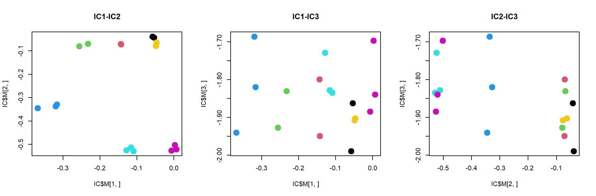
4.3.5. t-SNE
Unlike PCA, t-SNE shows not differences, but rather similarities. Similar objects should be located together. The method does not care about distant objects. The distance is weighted by Student (t) distribution (similar to Gaussian).
Let’s use Rtsne package. Please note, that when your
dataset is large, it is recommended to do PCA first before sending your
data to t-SNE. In Rtsne they use so called “Barnes-Hut
implementation” - faster but approximate.
#install.packages("Rtsne")
library(Rtsne)
## plot samples (not interesting)
TS1 = Rtsne(t(mRNA$X),perplexity=3,max_iter=2000)$Y
plot(TS1[,1],TS1[,2],col=as.integer(mRNA$meta$time),pch=19,cex=2, main="tSNE for samples (reducing gene space)")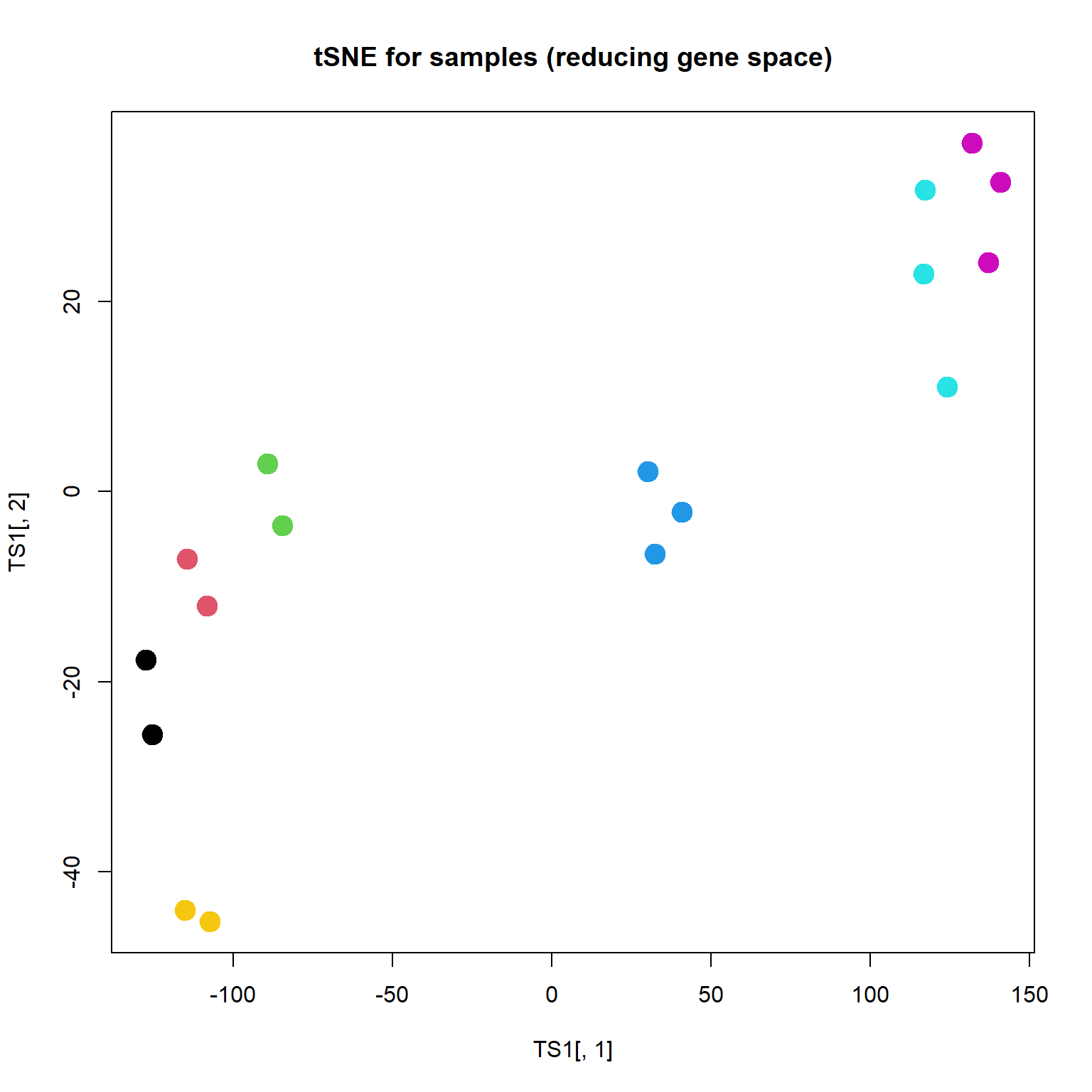
## plot features
TS2x = Rtsne(mRNA$X,perplexity=20,max_iter=1000,check_duplicates = FALSE )$Y
plot(TS2x[,1],TS2x[,2],col="#00AA0033",pch=19,cex=size, main="tSNE for genes (original)")
text(TS2x[genes,1],TS2x[genes,2],names(genes),col=1,pch=19,font=2)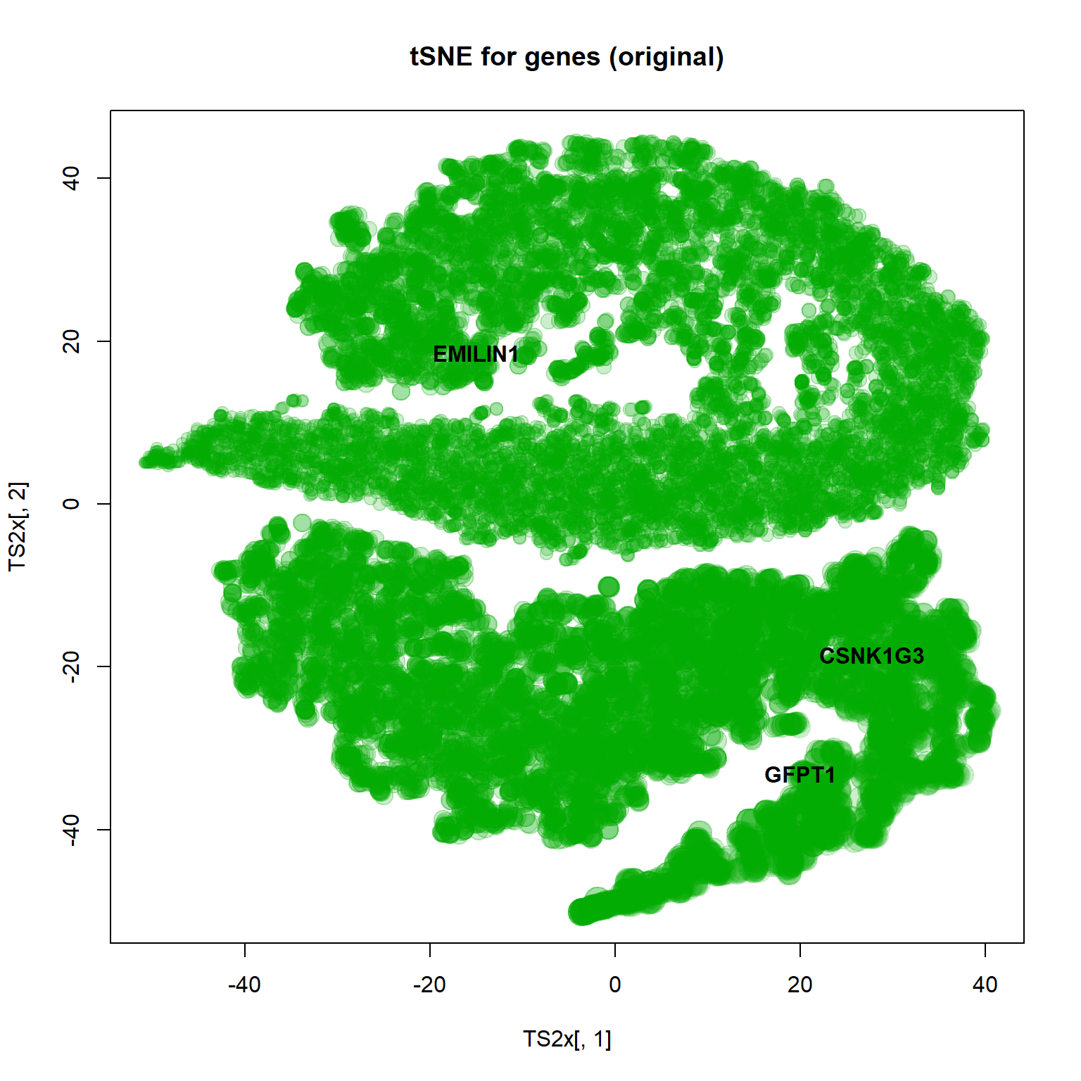
## same for scaled features (Z was calculated earlier)
TS2z = Rtsne(Z,perplexity=50,max_iter=1000,check_duplicates = FALSE)$Y
plot(TS2z[,1],TS2z[,2],col="#00AA0033",pch=19,cex=size, main="tSNE for genes (standardized genes)")
text(TS2z[genes,1],TS2z[genes,2],names(genes),col=1,pch=19,font=2)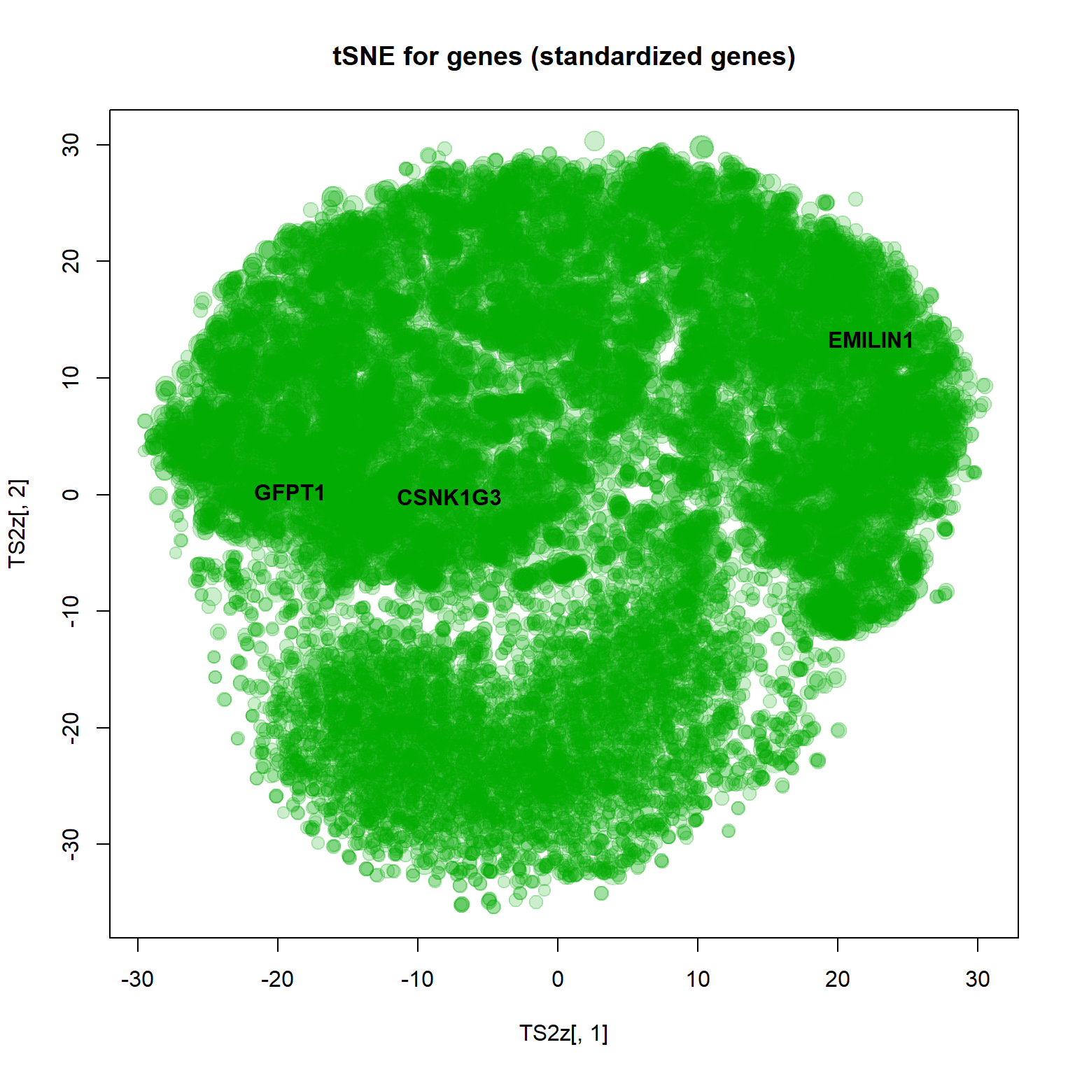
There is another package - tsne. It is
slower, but in some cases more precise. If “precise” can be used for
describing t-SNE ;)
4.4. STATISTICS in TRANSCRIPTOMICS
4.4.1. Linear models for transcriptomics data
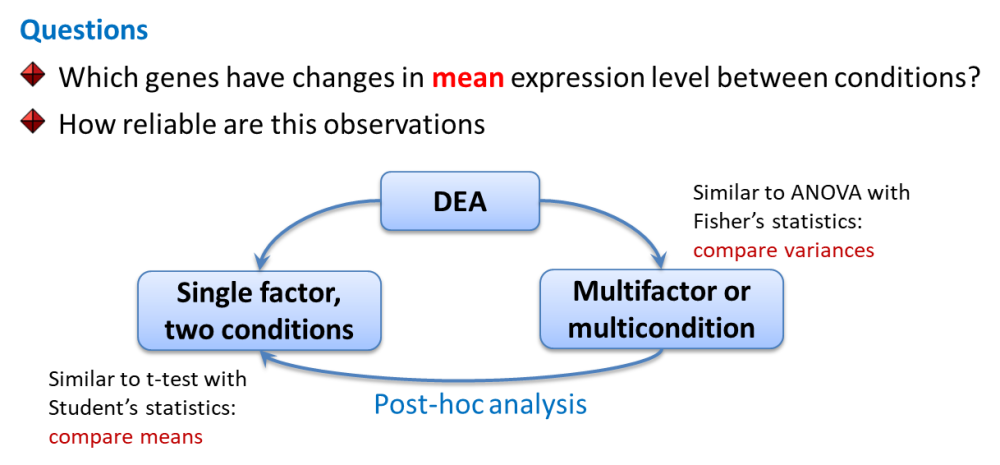
In genomics we will speak about differential expression analysis (DEA), when we would like to compare mean expression of genes between 2 or more sample groups.
4.4.2. DEA: Preparing for limma, edgeR, DESeq
In the native R, the vast majority of the libraries (or packages) can
be simply installed by install.libraries("library_name").
However, some advanced R/Bioconductor packages may need advanced
handling of the dependencies. Thus, we would recommend using
BiocManager::install() function:
if (!requireNamespace("BiocManager", quietly = TRUE))
    install.packages("BiocManager")

BiocManager::install("limma")
BiocManager::install("edgeR")
BiocManager::install("DESeq2")

## if you wish, you can also use my simple warp-up
source("http://r.modas.lu/LibDEA.r")
#DEA.limma
#DEA.edgeR
#DEA.DESeq
More detailed tutorials you could find on external resources, e.g.:
DESeq, or more correctly DESeq2,
(developed in EMBL, Heidelberg) is a very powerful package, but also the
most demanding one in terms of dependencies :)…
Please try to install all 3 packages.
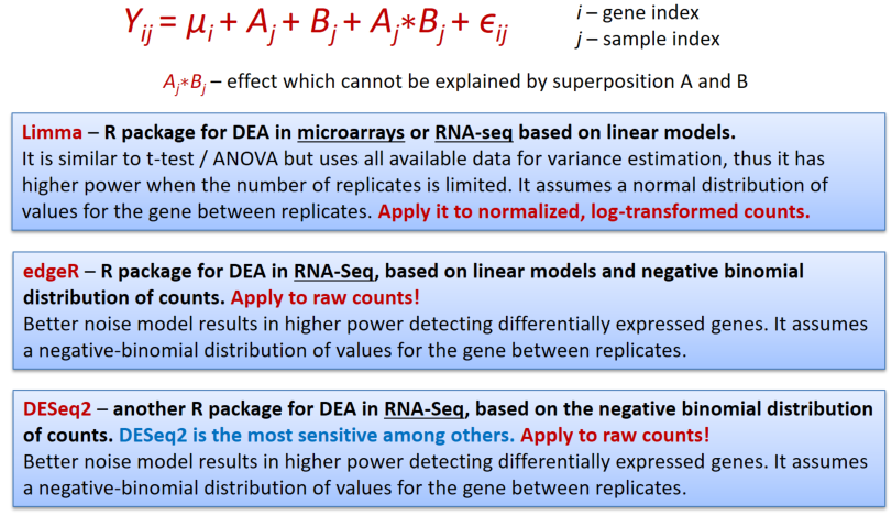
Limma works similar to ANOVA with somewhat improved post-hoc analysis and p-value calculation (empirical Bayes statistics).
4.4.2. DEA: Example of a time-course experiment
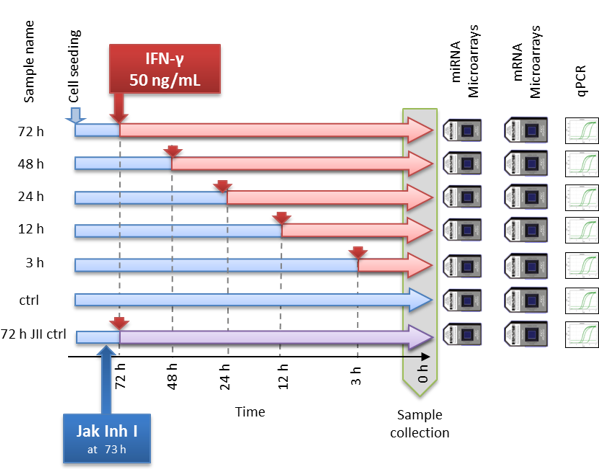
Let’s consider an example - a time course experiment from this paper.
This specific example is based on the microarray data, but all points
discussed below you can apply after to sequencing data using
corresponding warp-up: DEA.limma(...,counted=TRUE),
DEA.edgeR(...), DEA.DESeq(...).
Load the data from the following format
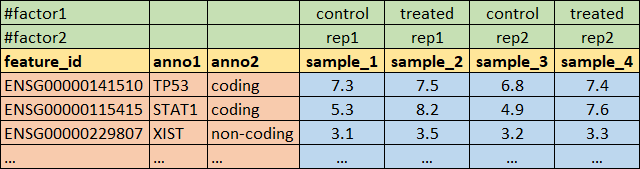
## load the data that are in annotated text format
source("http://r.modas.lu/readAMD.r")
mRNA = readAMD("http://edu.modas.lu/data/txt/mrna_ifng.amd.txt",
      stringsAsFactors=TRUE,
          index.column="GeneSymbol",
          sum.func="mean")
str(mRNA)
library(pheatmap)
## load custom functions
source("http://r.modas.lu/LibDEA.r")## [1] "----------------------------------------------------------------"
## [1] "libDEA: Differential expression analysis"
## [1] "Needed:"
## [1] "limma" "edgeR" "DESeq2" "caTools" "compiler" "sva"
## [1] "Absent:"
## character(0)## DEA: the most variable genes (by F-statistics)
ResF = DEA.limma(data = mRNA$X, group = mRNA$meta$time)## Loading required package: limma## [1] "T03-T00" "T12-T00" "T12-T03" "T24-T00" "T24-T03" "T24-T12"
## [7] "T48-T00" "T48-T03" "T48-T12" "T48-T24" "T72-T00" "T72-T03"
## [13] "T72-T12" "T72-T24" "T72-T48" "T72J-T00" "T72J-T03" "T72J-T12"
## [19] "T72J-T24" "T72J-T48" "T72J-T72"
##
## Limma,unpaired: 11468,9604,7444,5630 DEG (FDR<0.05, 1e-2, 1e-3, 1e-4)genes = order(ResF$FDR)[1:100] ## select top 100 genes
pheatmap(mRNA$X[genes,],cluster_col=FALSE,scale="row",
fontsize_row=2, fontsize_col=10, cellwidth=15,
main="Top 100 significant genes (F-stat)")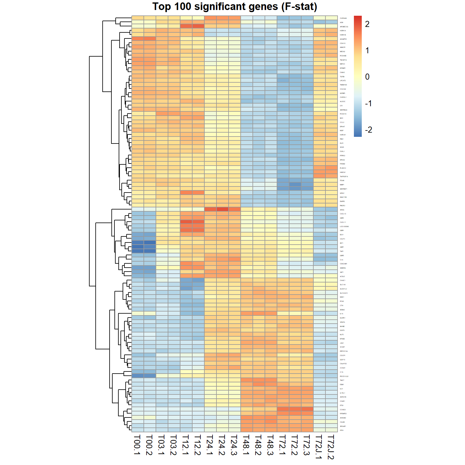
## DEA: genes differentially expressed (by moderated t-test)
Res24 = DEA.limma(data = mRNA$X,
                  group = mRNA$meta$time,
                  key0="T00",key1="T24")
##
## Limma,unpaired: 5895,3980,2146,1023 DEG (FDR<0.05, 1e-2, 1e-3, 1e-4)## volcano plot
plotVolcano(Res24,thr.fdr=0.01,thr.lfc=1)
genes = order(Res24$FDR)[1:100]  ## select top 100 genes
samples = grep("T00|T24",mRNA$meta$time) ## select T00,T24 sampl.
pheatmap(mRNA$X[genes,samples],cluster_col=FALSE,scale="row",
  fontsize_row=2, fontsize_col=10, cellwidth=15,
  main="Top 100 significant genes T24-T00 (moderated t-stat)")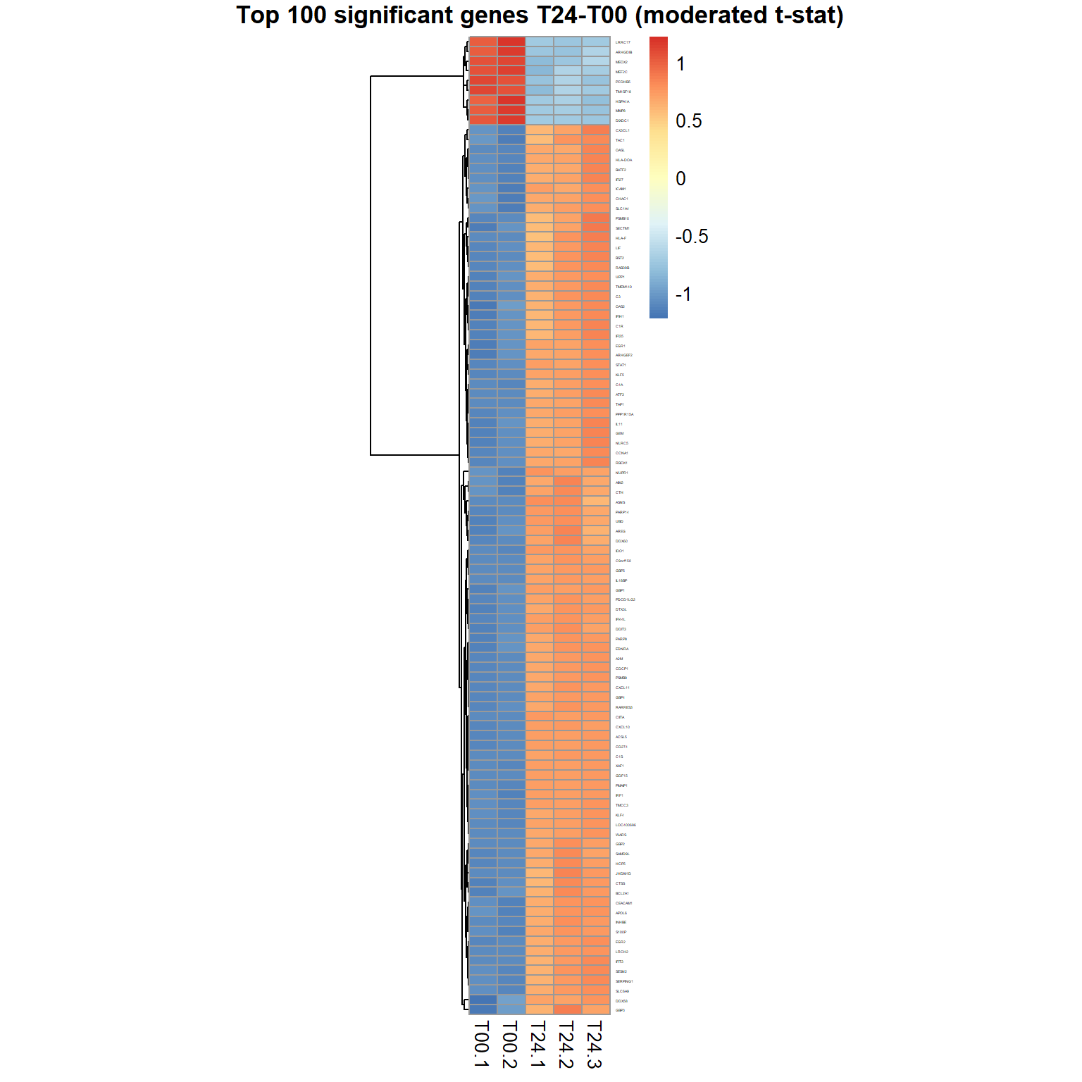
Let’s save the results - we will use the after for function annotation.
## save the most variable genes (by F-statistics)
write.table(ResF[ResF$FDR<0.0001,],file = "DEA_F.txt",
            col.names=NA, sep="\t", quote=FALSE)

## save significant genes T24-vs-T00
write.table(Res24[Res24$FDR<0.001 & abs(Res24$logFC)>1,],
            file = "DEA_T24-T00.txt",
            col.names=NA, sep="\t", quote=FALSE)
## save gene list (response at 24 h of IFNg treatment)
write(Res24[Res24$FDR<0.0001,1],file="genes24.txt")
Please, investigate the results. Submit any list to the functional annotation tool Enrichr
Other tools to be considered:
| Prev Home |
By Petr Nazarov
|