Lecture 2. Testing statistical hypotheses
Petr V. Nazarov, LIH
2024-02-19
| Materials: “Test:)” Presentation Tasks |
2.1. CONFIDENCE INTERVALS
2.1.1 Definitions
Interval estimate - An estimate of a population parameter that provides an interval believed to contain the value of the parameter. The interval estimates have the form: point estimate ± margin of error.
Margin of error - The ± value added to and subtracted from a point estimate in order to develop an interval estimate of a population parameter.
Confidence level - The confidence that is associated with an interval estimate. For example, if an interval estimation procedure provides intervals such that 95% of the intervals formed using the procedure will include the population parameter, the interval estimate is said to be constructed at the 95% confidence level. Confidence = 1 - \(\alpha\)
Confidence interval - Another name for an interval estimate.
Here the sampling distribution of the mean is shown by red normal curve. Population mean - green line. Experimentally observed sample mean (point estimate) - blue dot. Interval estimated - blue arrows.

2.1.2. Cofidence interval for mean (\(\sigma\)-known: normal)
When population st.deviation \(\sigma\) is known, we can build interval estimation using normal distribution.
Example An engineer is testing a new measuring device. He tries to put 500 µl of water into tubes and then measure the resulting quantity. Based on 36 measurements she estimated the average volume of 498 µl. From technical documentation for the device she learnt that the standard deviation of the volume is around 5 µl. Calculate the 95% and 99% confidence intervals for the volume the researcher takes on average. Is the desired volume of 500 µl in the confidence intervals?
m = 498    # observed mean
sigma = 5  # population st.dev
n = 36     # sample size
a = 0.05   # alpha for confidence 95%
me = -qnorm(a/2)*sigma/sqrt(n)
sprintf("mu = %g +/- %g",m,me)
## [1] "mu = 498 +/- 1.6333"2.1.3. Cofidence interval for mean (Student)
When population st.deviation \(\sigma\) is unknown, it is estimated from the sample. Then we should build interval estimation using Student’s t distribution.
You can use either calculate margin of error manually with
qt statistic or use t.test() (but then you
need data)
## manual calculation
m = 498    # observed mean
s = 5      # observed st.dev
n = 36     # sample size
a = 0.05   # alpha for confidence 95%
me = -qt(a/2,n-1)*s/sqrt(n)
sprintf("mu = %g +/- %g",m,me)
## [1] "mu = 498 +/- 1.69176"## using t.test() - need data. Here some random data are used
x = c(39,19,32,21,27,20,21,40,10)
t.test(x) # show##
## One Sample t-test
##
## data: x
## t = 7.6804, df = 8, p-value = 5.849e-05
## alternative hypothesis: true mean is not equal to 0
## 95 percent confidence interval:
## 17.80488 33.08401
## sample estimates:
## mean of x
## 25.44444t.test(x)$conf.int # gets conf.int## [1] 17.80488 33.08401
## attr(,"conf.level")
## [1] 0.952.1.4. Cofidence interval for proportion
Confidence interval for proportion is similar to C.I. for mean. In R you can use two functions
prop.test()that approximates errors with normal distribution (actually, x2 is used there) andbinom.test()which is exact test for binomial distribution. The former need large sample size. The latter should work with any number of observations.
Example: Studying a sample of 50 men, you observed 35 of them are overweight. Build interval estimate for proportion and check whether standard proportion of 40% overweight is within or outside of this interval.
## using prop.test
x = 35
n = 50
prop.test(x, n)
##
## 1-sample proportions test with continuity correction
##
## data: x out of n, null probability 0.5
## X-squared = 7.22, df = 1, p-value = 0.00721
## alternative hypothesis: true p is not equal to 0.5
## 95 percent confidence interval:
## 0.5521660 0.8171438
## sample estimates:
## p
## 0.7## using exact test
binom.test(x, n)##
## Exact binomial test
##
## data: x and n
## number of successes = 35, number of trials = 50, p-value = 0.0066
## alternative hypothesis: true probability of success is not equal to 0.5
## 95 percent confidence interval:
## 0.5539177 0.8213822
## sample estimates:
## probability of success
## 0.7Example Working with pancretitis dataset, define a 95% confidence interval for the proportion of never-smoking people coming to a hospital.
Pan = read.table("http://edu.modas.lu/data/txt/pancreatitis.txt", sep="\t", header=TRUE, stringsAsFactors = TRUE)

n = sum(Pan$Disease == "other")
x = sum(Pan$Smoking == "Never" & Pan$Disease == "other")
p = x/n
a = 0.05

# method 1: manual calculation
sp = sqrt(p*(1-p)/n)
me = -qnorm(a/2)*sp
sprintf("pi = %g +/- %g",p,me)
## [1] "pi = 0.258065 +/- 0.0582191"sprintf("pi = [%g, %g]",p-me,p+me)## [1] "pi = [0.199845, 0.316284]"# method 2: prop.test
prop.test(x,n,conf.level=1-a)$conf.int## [1] 0.2023108 0.3225644
## attr(,"conf.level")
## [1] 0.95# method 3: binom.test
binom.test(x,n,conf.level=1-a)$conf.int## [1] 0.2012123 0.3216558
## attr(,"conf.level")
## [1] 0.95Let’s calculate how many patients we would need to have error (E) less than 1
E = 0.01
n1 = qnorm(a/2)^2 * p * (1-p) / E^2
n1
## [1] 7355.1342.1.5. Interval estimates for random functions
In case you work with some functions over random observations, the shape of the distribution is difficult to get. You can use:
Numerical simulation
Special transformations (e.g.
logfor the ratio of strictly positive values)
Example Experimental values (x) and control (y) were measured for an experiment. 5 replicates were performed for each. From previous experience, we know that the error between replicates is not too different from normal distribution. Provide an interval estimation for the fold change x/y (alpha=0.05)
# enter the data
x = c(215,253,198,225,240)
y = c(83,75,62,91,70)

# means and standard errors
mx = mean(x)
my = mean(y)
sex = sd(x)/sqrt(5)
sey = sd(y)/sqrt(5)

# simulation (can try rnorm)
Mx = mx + sex*rt(10000,5-1)
My = my + sey*rt(10000,5-1)
FXY = Mx/My

# visualization
hist(FXY, 50, freq = FALSE)
lines(density(FXY),lwd=2,col=4)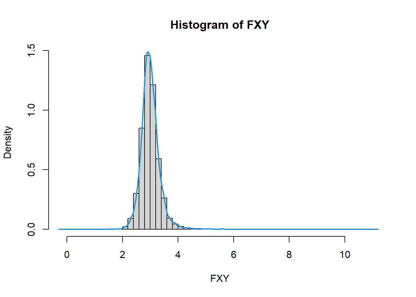
# confidence interval for means
quantile(Mx/My,c(0.025,0.975))
## 2.5% 97.5%
## 2.403044 3.752689Alternatively, in this speciffic case one could use log-transformation:
# use log-transformed data:
mx = mean(log2(x))
my = mean(log2(y))
sex = sd(log2(x))/sqrt(length(x))
sey = sd(log2(y))/sqrt(length(x))

m = mx - my
s = sqrt(sex^2 + sey^2)

me1 = m + qt(0.025,5-1)*s
me2 = m + qt(0.975,5-1)*s

## report exp:
sprintf("Mean m=%.2f has interval estimates [%.2f, %.2f]",2^m, 2^me1, 2^me2)
## [1] "Mean m=2.98 has interval estimates [2.40, 3.72]"2.2. HYPOTHESES FOR ONE SAMPLE
2.2.1. Hypotheses
Null hypothesis H0 - the hypothesis tentatively assumed true in the hypothesis testing procedure
Alternative hypothesis Ha - The hypothesis concluded to be true if the null hypothesis is rejected
Type I error, \(\alpha\) error. The error of rejecting H0 when it is true (inventing effect).
Type II error, \(\beta\) error. The error of accepting H0 when it is false (missing effect).
Level of significance. The probability of making a Type I error when the H0 is true as an equality, \(\alpha\)
p-value. A probability, computed using the test statistics, that measures the support (or lack of support) provided by the sample for the null hypothesis. It is a probability of making the error of Type I
2.2.2. Hypotheses about mean
Example A Trade Commission (TC) periodically conducts statistical studies designed to test the claims that manufacturers make about their products. For example, the label on a large can of Hilltop Coffee states that the can contains 3 pounds of coffee. The TC knows that Hilltop’s production process cannot place exactly 3 pounds of coffee in each can, even if the mean filling weight for the population of all cans filled is 3 pounds per can. However, as long as the population mean filling weight is at least 3 pounds per can, the rights of consumers will be protected. Thus, the TC interprets the label information on a large can of coffee as a claim by Hilltop that the population mean filling weight is at least 3 pounds per can. We will show how the TC can check Hilltop’s claim by conducting a lower tail hypothesis test.
mu0 = 3       # assumed population mean
m = 2.92      # observed sample mean
sigma = 0.18  # known population st.dev.
n = 36        # sample size

## standard error
se = sigma / sqrt(n)

## p-value
pnorm(m-mu0, mean = 0, sd = se)
## [1] 0.003830381Example The number of living cells in 5 wells under some conditions is given below, with an average value of 4705. In a reference literature source authors claimed a mean quantity of 5000 living cells under the same conditions. Is our result significantly different?
Cells: 5128,4806,5037,4231,4322
x = c(5128,4806,5037,4231,4322)

## one-tail hypothesis
pv1 = t.test(x, mu=5000,alternative="less")
pv1
##
## One Sample t-test
##
## data: x
## t = -1.612, df = 4, p-value = 0.09113
## alternative hypothesis: true mean is less than 5000
## 95 percent confidence interval:
## -Inf 5095.201
## sample estimates:
## mean of x
## 4704.8## two-tail hypothesis
pv2 = t.test(x, mu=5000,alternative ="two.sided")
pv2##
## One Sample t-test
##
## data: x
## t = -1.612, df = 4, p-value = 0.1823
## alternative hypothesis: true mean is not equal to 5000
## 95 percent confidence interval:
## 4196.355 5213.245
## sample estimates:
## mean of x
## 4704.82.2.3. Hypotheses about proportions
Example: Studying a sample of 50 men, you observed 35 of them are overweight. Test whether this proportion is significantly different from the standard proportion of 40% overweight.
## using prop.test
x = 35
n = 50
p = 0.4

prop.test(x, n, p)
##
## 1-sample proportions test with continuity correction
##
## data: x out of n, null probability p
## X-squared = 17.521, df = 1, p-value = 2.842e-05
## alternative hypothesis: true p is not equal to 0.4
## 95 percent confidence interval:
## 0.5521660 0.8171438
## sample estimates:
## p
## 0.7## using exact test
binom.test(x, n, p)##
## Exact binomial test
##
## data: x and n
## number of successes = 35, number of trials = 50, p-value = 3.104e-05
## alternative hypothesis: true probability of success is not equal to 0.4
## 95 percent confidence interval:
## 0.5539177 0.8213822
## sample estimates:
## probability of success
## 0.72.3. HYPOTHESES FOR TWO MEANS
Independent samples Samples are selected from two populations in such a way that the elements making up one sample are chosen independently of the elements making up the other sample.
Matched (paired) samples Samples, in which each data value of one sample is matched with a corresponding data value of the other sample.
2.3.1. Independent samples
Is the mean of weight change significantly different for males and females mice in mice dataset?
Mice = read.table("http://edu.modas.lu/data/txt/mice.txt", sep="\t", header=TRUE, stringsAsFactors = TRUE)

# slow way
x = Mice$Weight.change[Mice$Sex == "f"]
y = Mice$Weight.change[Mice$Sex == "m"]
t.test(x,y)
##
## Welch Two Sample t-test
##
## data: x and y
## t = -3.2067, df = 682.86, p-value = 0.001405
## alternative hypothesis: true difference in means is not equal to 0
## 95 percent confidence interval:
## -0.041059866 -0.009873477
## sample estimates:
## mean of x mean of y
## 1.093934 1.119401# fast way
t.test(Mice$Weight.change ~ Mice$Sex)##
## Welch Two Sample t-test
##
## data: Mice$Weight.change by Mice$Sex
## t = -3.2067, df = 682.86, p-value = 0.001405
## alternative hypothesis: true difference in means between group f and group m is not equal to 0
## 95 percent confidence interval:
## -0.041059866 -0.009873477
## sample estimates:
## mean in group f mean in group m
## 1.093934 1.119401#get p-value
tt = t.test(Mice$Weight.change ~ Mice$Sex)
tt$p.value## [1] 0.001405412.3.2. Matched samples
Example In the dataset bloodpressure, the systolic blood pressures of n=12 women between the ages of 20 and 35 were measured before and after usage of a newly developed oral contraceptive. Does the treatment affect the systolic blood pressure?
BP = read.table("http://edu.modas.lu/data/txt/bloodpressure.txt", sep="\t", header=TRUE, stringsAsFactors = TRUE)
t.test(BP$BP.before,  BP$BP.after, paired = TRUE)
##
## Paired t-test
##
## data: BP$BP.before and BP$BP.after
## t = -2.8976, df = 11, p-value = 0.01451
## alternative hypothesis: true mean difference is not equal to 0
## 95 percent confidence interval:
## -4.5455745 -0.6210921
## sample estimates:
## mean difference
## -2.5833332.3.3. Test for proportions
**Example* Consider 2 mouse strains SWR/J and MA/MyJ. Is the male proportion significantly different in these mouse strains (0.47 and 0.65)?
# no correction (approximate!):
prop.test(x = c(9,15),
          n = c(19,23),
          correct = FALSE)
##
## 2-sample test for equality of proportions without continuity correction
##
## data: c(9, 15) out of c(19, 23)
## X-squared = 1.3535, df = 1, p-value = 0.2447
## alternative hypothesis: two.sided
## 95 percent confidence interval:
## -0.4756308 0.1186514
## sample estimates:
## prop 1 prop 2
## 0.4736842 0.6521739# with correction:
prop.test(x = c(9,15),
n = c(19,23))##
## 2-sample test for equality of proportions with continuity correction
##
## data: c(9, 15) out of c(19, 23)
## X-squared = 0.72283, df = 1, p-value = 0.3952
## alternative hypothesis: two.sided
## 95 percent confidence interval:
## -0.5236857 0.1667063
## sample estimates:
## prop 1 prop 2
## 0.4736842 0.65217392.4. NON-PARAMETRIC TESTS
Non-parametric measures - statistical measures that do not depend on particular data distribution. Non-parametric tests are usually performed on ranks. Non-parametric procedures are more robust to outliers but less powerful than parametric ones
2.4.1 Unpaired test: Mann-Whitney-Wilcoxon U-test
Example Compare number of students in psychology and sociology directions:
Psy: 80,95,65,75,60,80,85,90,75,40
Soc: 90,30,65,60,55,70,70,35,75,30
psy = c(80,95,65,75,60,80,85,90,75,40)
soc = c(90,30,65,60,55,70,70,35,75,30)

wilcox.test(psy,soc)
## Warning in wilcox.test.default(psy, soc): cannot compute exact p-value with
## ties##
## Wilcoxon rank sum test with continuity correction
##
## data: psy and soc
## W = 76.5, p-value = 0.04851
## alternative hypothesis: true location shift is not equal to 02.4.1 Paired test: Wilcoxon Signed Rank Test
Example Compare an experimental measure done before and after treatment:
before: 12,42,31,462,1,25,63,754,12,34
after: 412,312,63,632,0,20,124,5356,83,1245
before = c(12,42,31,462,1,25,63,754,12,34)
after = c(412,312,63,632,0,20,124,5356,83,1245)

wilcox.test(before,after, paired = TRUE)
##
## Wilcoxon signed rank exact test
##
## data: before and after
## V = 3, p-value = 0.009766
## alternative hypothesis: true location shift is not equal to 02.5. MULTIPLE TESTING
False discovery rate (FDR) control is a statistical method used in multiple-hypothesis testing to correct for multiple comparisons. FDR controls the expected proportion of incorrectly rejected null hypotheses (type I errors) in a list of rejected hypotheses. FDR = FP / (FP + TP)
The family-wise error rate (FWER) is the probability of making one or more false discoveries, or type I errors, when performing multiple hypothesis tests. It is calculated as the probability of rejecting at least one true null hypothesis out of all the hypotheses tested. FWER = P(FP ≥ 1). It is stricter than FDR
Example Let’s generate 6 columns of normal random variables (1000 points/candidates in each). Consider the first 3 columns as “treatment”, and the next 3 columns as “control”. Using t-test calculate p-values b/w “treatment” and “control” group. How many candidates have p-value<0.05 ? Calculate FDR/FWER. How many candidates you have now?
# create dataset
X = matrix(rnorm(1000*6), nrow=1000, ncol=6)

# test 1000 hypotheses
pv = 1
for (i in 1:nrow(X)){
  res=t.test(X[i,1:3], X[i,4:6])
  pv[i]=res$p.value
}

# number of pv < 0.05
sum(pv<0.05)
## [1] 29# FDR adjustment
fdr = p.adjust(pv,"fdr")
sum(fdr<0.05)## [1] 0# FWER adjustment
fwer = p.adjust(pv,"holm")
sum(fwer<0.05)## [1] 0| Prev Home Next |
By Petr Nazarov
|