3. Statistical basics
Petr V. Nazarov, LIH
2023-10-24
3.1. Hypothesis testing and p-value
Here are few slides explaining the concept of hypothesis testing and p-value:
As an example, let’s do hypothesis testing from the lecture.
mu0 = 3   ## constant to which we compare
m = 2.92  ## experimentally observed mean weight
s = 0.18  ## standard deviation (known in advance)
n = 36    ## number of observations

## standard error (st.dev of mean)
sm = s/sqrt(n)

## statistics
z = (m-mu0)/sm

## p-value
pnorm(z)
## [1] 0.0038303813.2. Multiple testing
Let’s run a small test described in the lecture: generate a random dataset with 1000 “genes” for 6 “samples”. 3 samples we denote as “A”, 3 - as “B”.
library(pheatmap)

ng = 1000  ## n genes
nr = 3     ## n replicates

## random matrix
X = matrix(rnorm(ng*nr*2),nrow=ng, ncol=nr*2)
rownames(X) = paste0("gene",1:ng)
colnames(X) = c(paste0("A",1:nr),paste0("B",1:nr))
pheatmap(X,fontsize_row = 1,cellwidth=20,main="Random expression matrix",scale="row")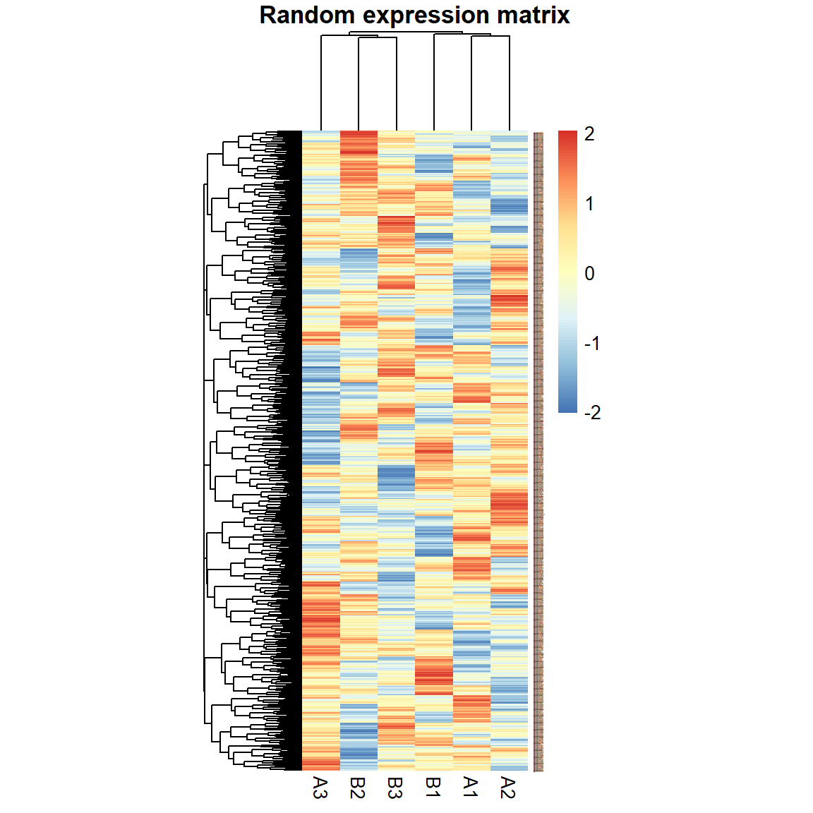
## calculate p-values
pv = double(ng)
names(pv) = rownames(X)
for (i in 1:ng){
  pv[i] = t.test(X[i,1:nr],X[i,(nr+1):(2*nr)])$p.value
}
pheatmap(X[pv<0.05,],cellwidth=20,main="Significant genes by p-value",scale="row")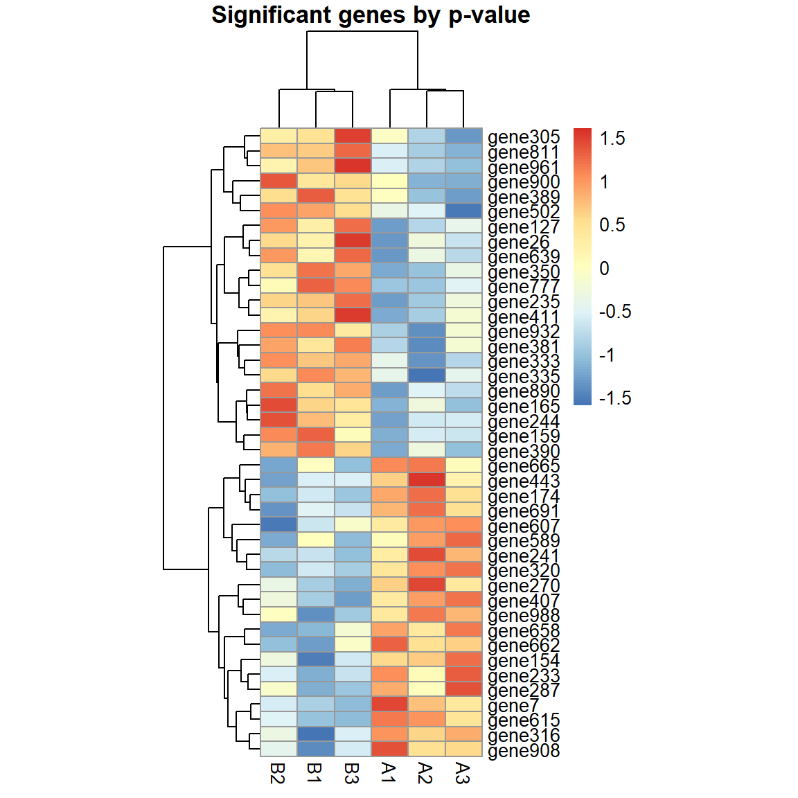
## Significant genes by p-value:
print(names(pv)[pv<0.05])
## [1] "gene7" "gene26" "gene127" "gene154" "gene159" "gene165" "gene174"
## [8] "gene233" "gene235" "gene241" "gene244" "gene270" "gene287" "gene305"
## [15] "gene316" "gene320" "gene333" "gene335" "gene350" "gene381" "gene389"
## [22] "gene390" "gene407" "gene411" "gene443" "gene502" "gene589" "gene607"
## [29] "gene615" "gene639" "gene658" "gene662" "gene665" "gene691" "gene777"
## [36] "gene811" "gene890" "gene900" "gene908" "gene932" "gene961" "gene988"## Correction for multiple testing using Benjamini-Hochberg's FDR and Holm's FWER
fdr = p.adjust(pv,"fdr")
fwer = p.adjust(pv,"holm")
## Significant genes by FDR:
print(names(fdr)[fdr<0.05])## character(0)data.frame(PV=pv[pv<0.05],FDR=fdr[pv<0.05],FWER=fwer[pv<0.05])## PV FDR FWER
## gene7 0.021895544 0.989248 1
## gene26 0.041042683 0.989248 1
## gene127 0.012037702 0.989248 1
## gene154 0.027464496 0.989248 1
## gene159 0.033390591 0.989248 1
## gene165 0.017466140 0.989248 1
## gene174 0.004353100 0.989248 1
## gene233 0.031262568 0.989248 1
## gene235 0.014661714 0.989248 1
## gene241 0.025810482 0.989248 1
## gene244 0.016646933 0.989248 1
## gene270 0.019494766 0.989248 1
## gene287 0.047597156 0.989248 1
## gene305 0.046156357 0.989248 1
## gene316 0.037715157 0.989248 1
## gene320 0.008339019 0.989248 1
## gene333 0.018099005 0.989248 1
## gene335 0.041418773 0.989248 1
## gene350 0.006252510 0.989248 1
## gene381 0.024999367 0.989248 1
## gene389 0.037631536 0.989248 1
## gene390 0.009785195 0.989248 1
## gene407 0.013981557 0.989248 1
## gene411 0.044237857 0.989248 1
## gene443 0.037343756 0.989248 1
## gene502 0.034716690 0.989248 1
## gene589 0.045941882 0.989248 1
## gene607 0.044047356 0.989248 1
## gene615 0.004249717 0.989248 1
## gene639 0.022515987 0.989248 1
## gene658 0.018295086 0.989248 1
## gene662 0.029860376 0.989248 1
## gene665 0.042668367 0.989248 1
## gene691 0.008856648 0.989248 1
## gene777 0.033385631 0.989248 1
## gene811 0.002621773 0.989248 1
## gene890 0.004870564 0.989248 1
## gene900 0.040357883 0.989248 1
## gene908 0.017962831 0.989248 1
## gene932 0.023623322 0.989248 1
## gene961 0.044919353 0.989248 1
## gene988 0.041295880 0.989248 13.3. Analysis of Variance (ANOVA)
Here are few slides explaining the problems of multiple hypothesis testing and the concept of ANOVA: analysis of variance.
Multiple testing, ANOVA Partek’s ANOVA
As an example, you could consider depression measured in healthy and sick respondents in 3 locations: California, New York and North Carolina.
## load data
Dep = read.table("http://edu.modas.lu/data/txt/depression2.txt",header=T,sep="\t",as.is=FALSE)
str(Dep)
## 'data.frame': 120 obs. of 3 variables:
## $ Location : Factor w/ 3 levels "Florida","New York",..: 1 1 1 1 1 1 1 1 1 1 ...
## $ Health : Factor w/ 2 levels "bad","good": 2 2 2 2 2 2 2 2 2 2 ...
## $ Depression: int 3 7 7 3 8 8 8 5 5 2 ...3.3.1. One-way (one-factor) ANOVA
We start with one-way ANOVA. Let’s consider only healthy respondents
in Dep dataset. ANOVA is performed in R:
aov(formula, data)
formula- “Values ~ Factor1”, where “Values”, “Factor1” should be replaced by the actual column names in the data framedata
ANOVA tells whether a factor is significant, but tells nothing with
treatments (factor levels) are different! Use TukeyHSD() to
perform post-hoc analysis and get corrected p-values for the
contrasts.
DepGH = Dep[Dep$Health == "good",]

## build 1-factor ANOVA model
res1 = aov(Depression ~  Location, DepGH)
summary(res1)
## Df Sum Sq Mean Sq F value Pr(>F)
## Location 2 78.5 39.27 6.773 0.0023 **
## Residuals 57 330.4 5.80
## ---
## Signif. codes: 0 '***' 0.001 '**' 0.01 '*' 0.05 '.' 0.1 ' ' 1TukeyHSD(res1)## Tukey multiple comparisons of means
## 95% family-wise confidence level
##
## Fit: aov(formula = Depression ~ Location, data = DepGH)
##
## $Location
## diff lwr upr p adj
## New York-Florida 2.8 0.9677423 4.6322577 0.0014973
## North Carolina-Florida 1.5 -0.3322577 3.3322577 0.1289579
## North Carolina-New York -1.3 -3.1322577 0.5322577 0.21126123.3.2. Two-way (two-factor) ANOVA
For two-way ANOVA the call is similar
aov(formula, data). Please note that factor columns in the
data frame data should be of class "factor"
(newer R version accepts "character"). If factors are
"numeric", aov will build regression instead.
formula- “Values ~ Factor1 + Factor2 + Factor1*Factor2”, where “Values”, “Factor1” and “Factor2” should be replaced by the actual column names in the data framedataInteraction “Factor1*Factor2” can be estimated in case, if you table contains replicates (values measured for the same conditions)
If needed, ANOVA can be followed by TukeyHSD().
## build 2-factor ANOVA model (with interaction)
res2 = aov(Depression ~  Location + Health + Location*Health, Dep)
summary(res2)
## Df Sum Sq Mean Sq F value Pr(>F)
## Location 2 73.8 36.9 4.290 0.016 *
## Health 1 1748.0 1748.0 203.094 <2e-16 ***
## Location:Health 2 26.1 13.1 1.517 0.224
## Residuals 114 981.2 8.6
## ---
## Signif. codes: 0 '***' 0.001 '**' 0.01 '*' 0.05 '.' 0.1 ' ' 1TukeyHSD(res2)## Tukey multiple comparisons of means
## 95% family-wise confidence level
##
## Fit: aov(formula = Depression ~ Location + Health + Location * Health, data = Dep)
##
## $Location
## diff lwr upr p adj
## New York-Florida 1.850 0.2921599 3.4078401 0.0155179
## North Carolina-Florida 0.475 -1.0828401 2.0328401 0.7497611
## North Carolina-New York -1.375 -2.9328401 0.1828401 0.0951631
##
## $Health
## diff lwr upr p adj
## good-bad -7.633333 -8.694414 -6.572252 0
##
## $`Location:Health`
## diff lwr upr p adj
## New York:bad-Florida:bad 0.90 -1.7893115 3.589311 0.9264595
## North Carolina:bad-Florida:bad -0.55 -3.2393115 2.139311 0.9913348
## Florida:good-Florida:bad -8.95 -11.6393115 -6.260689 0.0000000
## New York:good-Florida:bad -6.15 -8.8393115 -3.460689 0.0000000
## North Carolina:good-Florida:bad -7.45 -10.1393115 -4.760689 0.0000000
## North Carolina:bad-New York:bad -1.45 -4.1393115 1.239311 0.6244461
## Florida:good-New York:bad -9.85 -12.5393115 -7.160689 0.0000000
## New York:good-New York:bad -7.05 -9.7393115 -4.360689 0.0000000
## North Carolina:good-New York:bad -8.35 -11.0393115 -5.660689 0.0000000
## Florida:good-North Carolina:bad -8.40 -11.0893115 -5.710689 0.0000000
## New York:good-North Carolina:bad -5.60 -8.2893115 -2.910689 0.0000003
## North Carolina:good-North Carolina:bad -6.90 -9.5893115 -4.210689 0.0000000
## New York:good-Florida:good 2.80 0.1106885 5.489311 0.0361494
## North Carolina:good-Florida:good 1.50 -1.1893115 4.189311 0.5892328
## North Carolina:good-New York:good -1.30 -3.9893115 1.389311 0.7262066Take home messages 3
- When doing multiple hypothesis testing and selecting only those elements which are significant – always use FDR (or other, like FWER) correction!
- DEA provides the genes which have variability in mean gene expression between condition
- =>more data you have, the smaller differences you will be able to see
- Several factors can be taken into account in ANOVA approach. This will give you insight into the significance of each experimental factor but at the same time will correct batch effects and allow answering complex questions (remember shoes affecting ladies…).
| Prev Home Next |
By Petr Nazarov
|