3. Survival analysis
Petr V. Nazarov, LIH
2024-10-28
3.1 Survival data and survival analysis
Survival analysis is a branch of statistics which deals with analysis of time to events, such as death in biological organisms and failure in mechanical systems (i.e. reliability theory in engineering).
Survival analysis attempts to answer questions such as:
What is the proportion of a population which will survive past a certain time?
Of those that survive, at what rate will they die or fail?
Can multiple causes of death or failure be taken into account?
How do particular circumstances or characteristics increase or decrease the probability of survival?
Survival data include:
- Time-to-event: The duration from the start of the study until an event of interest occurs (such as death) or until the subject is censored (for example, if the patient withdraws from the study).
- Censoring status: A variable indicating whether the endpoint was observed (1 for the event occurrence) or censored (0 for non-occurrence due to end of study period or withdrawal).
- Predictor variables: Various factors or covariates that may influence the time to the event, which can be continuous or categorical in nature.
library(survival)
str(lung)
## 'data.frame': 228 obs. of 10 variables:
## $ inst : num 3 3 3 5 1 12 7 11 1 7 ...
## $ time : num 306 455 1010 210 883 ...
## $ status : num 2 2 1 2 2 1 2 2 2 2 ...
## $ age : num 74 68 56 57 60 74 68 71 53 61 ...
## $ sex : num 1 1 1 1 1 1 2 2 1 1 ...
## $ ph.ecog : num 1 0 0 1 0 1 2 2 1 2 ...
## $ ph.karno : num 90 90 90 90 100 50 70 60 70 70 ...
## $ pat.karno: num 100 90 90 60 90 80 60 80 80 70 ...
## $ meal.cal : num 1175 1225 NA 1150 NA ...
## $ wt.loss : num NA 15 15 11 0 0 10 1 16 34 ...## create a survival object
## lung$status: 1-censored, 2-dead
sData = Surv(lung$time, event = lung$status == 2)
print(sData)## [1] 306 455 1010+ 210 883 1022+ 310 361 218 166 170 654
## [13] 728 71 567 144 613 707 61 88 301 81 624 371
## [25] 394 520 574 118 390 12 473 26 533 107 53 122
## [37] 814 965+ 93 731 460 153 433 145 583 95 303 519
## [49] 643 765 735 189 53 246 689 65 5 132 687 345
## [61] 444 223 175 60 163 65 208 821+ 428 230 840+ 305
## [73] 11 132 226 426 705 363 11 176 791 95 196+ 167
## [85] 806+ 284 641 147 740+ 163 655 239 88 245 588+ 30
## [97] 179 310 477 166 559+ 450 364 107 177 156 529+ 11
## [109] 429 351 15 181 283 201 524 13 212 524 288 363
## [121] 442 199 550 54 558 207 92 60 551+ 543+ 293 202
## [133] 353 511+ 267 511+ 371 387 457 337 201 404+ 222 62
## [145] 458+ 356+ 353 163 31 340 229 444+ 315+ 182 156 329
## [157] 364+ 291 179 376+ 384+ 268 292+ 142 413+ 266+ 194 320
## [169] 181 285 301+ 348 197 382+ 303+ 296+ 180 186 145 269+
## [181] 300+ 284+ 350 272+ 292+ 332+ 285 259+ 110 286 270 81
## [193] 131 225+ 269 225+ 243+ 279+ 276+ 135 79 59 240+ 202+
## [205] 235+ 105 224+ 239 237+ 173+ 252+ 221+ 185+ 92+ 13 222+
## [217] 192+ 183 211+ 175+ 197+ 203+ 116 188+ 191+ 105+ 174+ 177+3.2 Kaplan-Meier plot
Visualization can be done using Kaplan-Meier plot
## visualize it using Kaplan-Meier plot
fit = survfit(sData ~ 1)
plot(fit, conf.int = TRUE, xlab="Time, days", ylab="Survived proportion")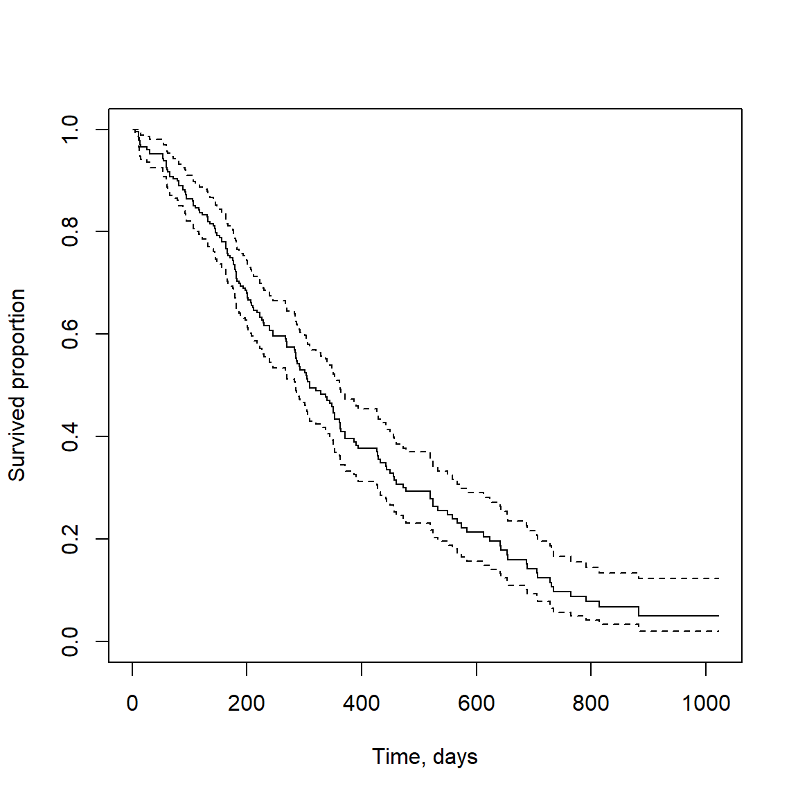
This can be also done for several subgroups:
## visualize for groups: male=1 / female=2
fit.sex = survfit(sData ~ lung$sex)
plot(fit.sex, col=c("blue","red"), mark.time=TRUE, xlab="Time, days", ylab="Survived proportion")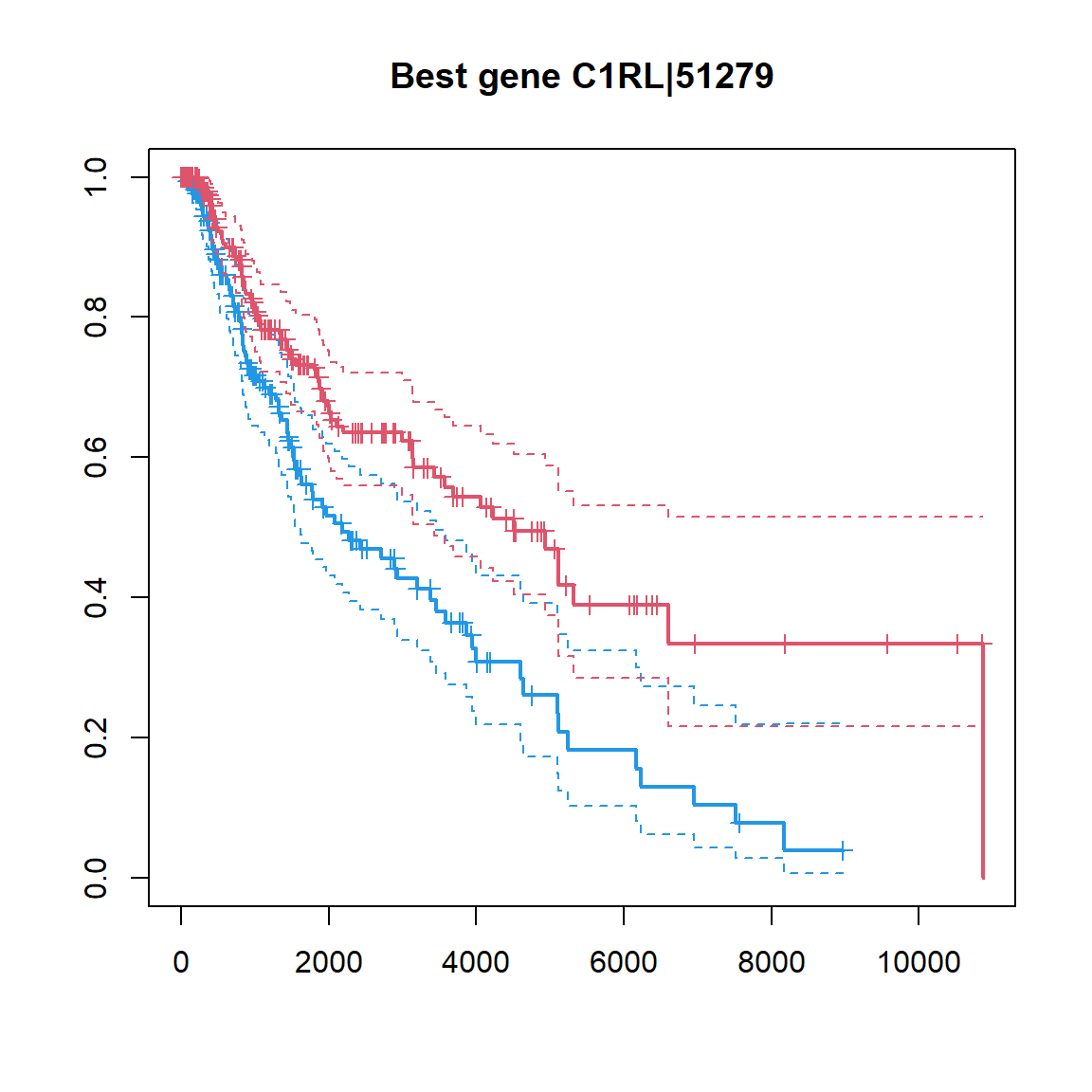
3.3. Cox model
Cox proportional hazards model, a.k.a. Cox model or Cox regression, is a statistical technique used in survival analysis. It models the time it takes for a certain event, like death, to occur as a function of predictor variables, without need to specify the form of the baseline hazard function. This allows for the estimation of the effect of the predictor variables on the hazard, or the event rate, at any given time.
Hazard function \(h(t)\) depends on basic hazard \(h_0(t)\) and variables \(x_1,..,x_n\):
\[h(t) = h_0(t) \times e^{\beta_1x_1+\beta_2x_2+...+\beta_nx_n} \] here \(\beta_i\) are fitted variables.
Hazard ratio (HR): \[HR = \frac{h_A(t)}{h_B(t)} = \exp{[\beta_1(x_{A1}-x_{B1}) + ... + \beta_n(x_{An}-x_{Bn})]}\] Working with log hazard ratio (LHR) makes life a bit easier. :)
\[LHR = \log({h_A(t)}) - \log({h_B(t)}) =
\beta_1(x_{A1}-x_{B1}) + ... + \beta_n(x_{An}-x_{Bn})\] Let’s
build Cox regression for lung data using a single variable
- sex
coxmod1 = coxph(sData ~ sex, data=lung)
summary(coxmod1)
## Call:
## coxph(formula = sData ~ sex, data = lung)
##
## n= 228, number of events= 165
##
## coef exp(coef) se(coef) z Pr(>|z|)
## sex -0.5310 0.5880 0.1672 -3.176 0.00149 **
## ---
## Signif. codes: 0 '***' 0.001 '**' 0.01 '*' 0.05 '.' 0.1 ' ' 1
##
## exp(coef) exp(-coef) lower .95 upper .95
## sex 0.588 1.701 0.4237 0.816
##
## Concordance= 0.579 (se = 0.021 )
## Likelihood ratio test= 10.63 on 1 df, p=0.001
## Wald test = 10.09 on 1 df, p=0.001
## Score (logrank) test = 10.33 on 1 df, p=0.001## build Cox regression model with 2 variables
mod2 = coxph(sData ~ sex + age, data=lung)
summary(mod2)## Call:
## coxph(formula = sData ~ sex + age, data = lung)
##
## n= 228, number of events= 165
##
## coef exp(coef) se(coef) z Pr(>|z|)
## sex -0.513219 0.598566 0.167458 -3.065 0.00218 **
## age 0.017045 1.017191 0.009223 1.848 0.06459 .
## ---
## Signif. codes: 0 '***' 0.001 '**' 0.01 '*' 0.05 '.' 0.1 ' ' 1
##
## exp(coef) exp(-coef) lower .95 upper .95
## sex 0.5986 1.6707 0.4311 0.8311
## age 1.0172 0.9831 0.9990 1.0357
##
## Concordance= 0.603 (se = 0.025 )
## Likelihood ratio test= 14.12 on 2 df, p=9e-04
## Wald test = 13.47 on 2 df, p=0.001
## Score (logrank) test = 13.72 on 2 df, p=0.001## build multivariable Cox regression model (can be problematic!)
mod3 = coxph(sData ~ ., data=lung[,-(1:3)])
summary(mod3)## Call:
## coxph(formula = sData ~ ., data = lung[, -(1:3)])
##
## n= 168, number of events= 121
## (60 observations deleted due to missingness)
##
## coef exp(coef) se(coef) z Pr(>|z|)
## age 1.065e-02 1.011e+00 1.161e-02 0.917 0.35906
## sex -5.509e-01 5.765e-01 2.008e-01 -2.743 0.00609 **
## ph.ecog 7.342e-01 2.084e+00 2.233e-01 3.288 0.00101 **
## ph.karno 2.246e-02 1.023e+00 1.124e-02 1.998 0.04574 *
## pat.karno -1.242e-02 9.877e-01 8.054e-03 -1.542 0.12316
## meal.cal 3.329e-05 1.000e+00 2.595e-04 0.128 0.89791
## wt.loss -1.433e-02 9.858e-01 7.771e-03 -1.844 0.06518 .
## ---
## Signif. codes: 0 '***' 0.001 '**' 0.01 '*' 0.05 '.' 0.1 ' ' 1
##
## exp(coef) exp(-coef) lower .95 upper .95
## age 1.0107 0.9894 0.9880 1.0340
## sex 0.5765 1.7347 0.3889 0.8545
## ph.ecog 2.0838 0.4799 1.3452 3.2277
## ph.karno 1.0227 0.9778 1.0004 1.0455
## pat.karno 0.9877 1.0125 0.9722 1.0034
## meal.cal 1.0000 1.0000 0.9995 1.0005
## wt.loss 0.9858 1.0144 0.9709 1.0009
##
## Concordance= 0.651 (se = 0.029 )
## Likelihood ratio test= 28.33 on 7 df, p=2e-04
## Wald test = 27.58 on 7 df, p=3e-04
## Score (logrank) test = 28.41 on 7 df, p=2e-04We cannot visualize directly Cox model with Kaplan-Meier. You have to use univariable model with categorization of the variable.
## Vizualize results of the Cox regression (univariable)
mod4 = coxph(sData ~ ph.ecog, data=lung)
summary(mod4)
## Call:
## coxph(formula = sData ~ ph.ecog, data = lung)
##
## n= 227, number of events= 164
## (1 observation deleted due to missingness)
##
## coef exp(coef) se(coef) z Pr(>|z|)
## ph.ecog 0.4759 1.6095 0.1134 4.198 2.69e-05 ***
## ---
## Signif. codes: 0 '***' 0.001 '**' 0.01 '*' 0.05 '.' 0.1 ' ' 1
##
## exp(coef) exp(-coef) lower .95 upper .95
## ph.ecog 1.61 0.6213 1.289 2.01
##
## Concordance= 0.604 (se = 0.024 )
## Likelihood ratio test= 17.57 on 1 df, p=3e-05
## Wald test = 17.62 on 1 df, p=3e-05
## Score (logrank) test = 17.89 on 1 df, p=2e-05fact = as.integer(lung$ph.ecog > median(lung$ph.ecog, na.rm = TRUE))
fact = factor(c("low","high")[fact+1],levels=c("low","high"))
fit.ph.ecog = survfit(sData ~ fact)
plot(fit.ph.ecog, col=c("blue","red"), mark.time=TRUE, xlab="Time, days", ylab="Survived", main="ph.ecog score low and high")
legend("topright",c("ph.ecog < median","ph.ecog > median"),col=c("blue","red"),lty=1)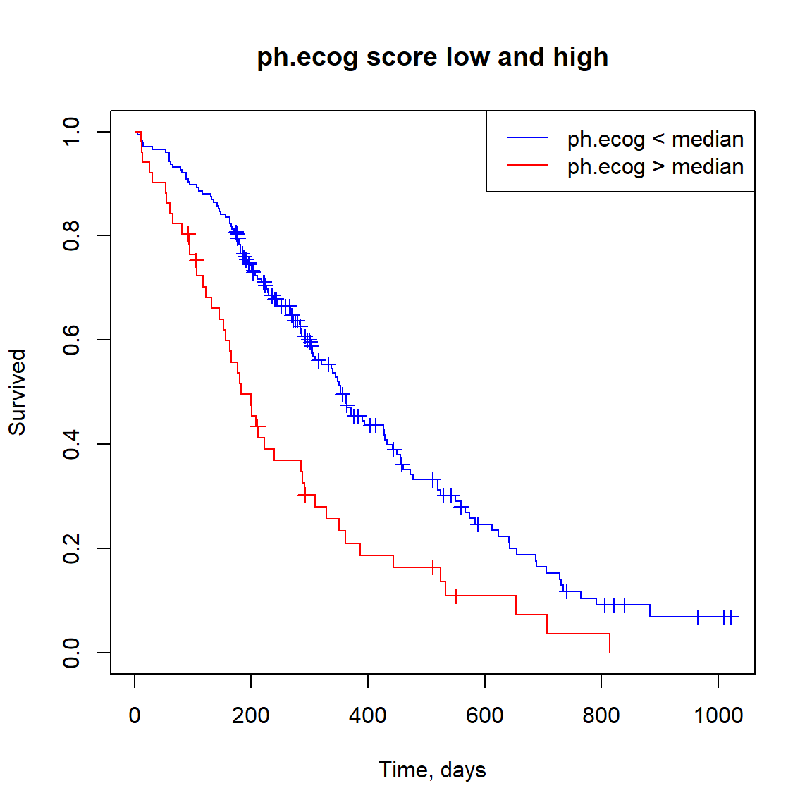
3.4. Survival analysis in omics: combining variables
Now let’s take transcriptomics dataset from TCGA: melanoma (SKCM)
Download data:
library(survival)
download.file("http://edu.modas.lu/data/rda/SKCM.RData","SKCM.RData",mode="wb")
load("SKCM.RData")
str(Data)
Now, let’s work with the dataset.
str(Data)## List of 6
## $ ns : int 473
## $ nf : int 20531
## $ anno.file: chr "D:/Data/TCGA/TCGA.hg19.June2011.gaf"
## $ anno :'data.frame': 20531 obs. of 2 variables:
## ..$ gene : chr [1:20531] "?|100130426" "?|100133144" "?|100134869" "?|10357" ...
## ..$ location: chr [1:20531] "chr9:79791679-79792806:+" "chr15:82647286-82708202:+;chr15:83023773-83084727:+" "chr15:82647286-82707815:+;chr15:83023773-83084340:+" "chr20:56063450-56064083:-" ...
## $ meta :'data.frame': 473 obs. of 61 variables:
## ..$ data.files : chr [1:473] "unc.edu.00624286-41dd-476f-a63b-d2a5f484bb45.2250155.rsem.genes.results" "unc.edu.01c6644f-c721-4f5e-afbc-c220218941d8.2557685.rsem.genes.results" "unc.edu.020f448b-0242-4ff7-912a-4598d0b49055.1211973.rsem.genes.results" "unc.edu.02486980-eb4f-4930-ba27-356e346929b6.1677015.rsem.genes.results" ...
## ..$ barcode : chr [1:473] "TCGA-GN-A4U7-06A-21R-A32P-07" "TCGA-W3-AA1V-06B-11R-A40A-07" "TCGA-FS-A1Z0-06A-11R-A18T-07" "TCGA-D9-A3Z1-06A-11R-A239-07" ...
## ..$ disease : chr [1:473] "SKCM" "SKCM" "SKCM" "SKCM" ...
## ..$ sample_type : chr [1:473] "TM" "TM" "TM" "TM" ...
## ..$ center : chr [1:473] "UNC-LCCC" "UNC-LCCC" "UNC-LCCC" "UNC-LCCC" ...
## ..$ platform : chr [1:473] "ILLUMINA" "ILLUMINA" "ILLUMINA" "ILLUMINA" ...
## ..$ aliquot_id : chr [1:473] "00624286-41dd-476f-a63b-d2a5f484bb45" "01c6644f-c721-4f5e-afbc-c220218941d8" "020f448b-0242-4ff7-912a-4598d0b49055" "02486980-eb4f-4930-ba27-356e346929b6" ...
## ..$ participant_id : chr [1:473] "088c296e-8e13-4dc8-8a99-b27f4b27f95e" "9817ec15-605a-40db-b848-2199e5ccbb7b" "6a1966c3-7f01-4304-b4a1-c4ef683b179a" "4f7e7a0e-4aa2-4b6a-936f-6429c7d6a2a7" ...
## ..$ sample_type_name : Factor w/ 4 levels "Additional Metastatic",..: 2 2 2 2 2 2 3 2 2 2 ...
## ..$ bcr_patient_uuid : chr [1:473] "088C296E-8E13-4DC8-8A99-B27F4B27F95E" "9817EC15-605A-40DB-B848-2199E5CCBB7B" "6A1966C3-7F01-4304-B4A1-C4EF683B179A" "4F7E7A0E-4AA2-4B6A-936F-6429C7D6A2A7" ...
## ..$ bcr_patient_barcode : chr [1:473] "TCGA-GN-A4U7" "TCGA-W3-AA1V" "TCGA-FS-A1Z0" "TCGA-D9-A3Z1" ...
## ..$ form_completion_date : chr [1:473] "2013-8-19" "2014-7-17" "2012-11-12" "2012-7-24" ...
## ..$ prospective_collection : Factor w/ 2 levels "NO","YES": 1 1 1 2 1 2 2 1 1 1 ...
## ..$ retrospective_collection : Factor w/ 2 levels "NO","YES": 2 2 2 1 2 1 1 2 2 2 ...
## ..$ birth_days_to : num [1:473] -20458 -23314 -11815 -24192 -16736 ...
## ..$ gender : Factor w/ 2 levels "FEMALE","MALE": 1 2 1 2 2 1 2 2 1 2 ...
## ..$ height_cm_at_diagnosis : num [1:473] 161 180 NA 180 NA 160 173 182 NA NA ...
## ..$ weight_kg_at_diagnosis : num [1:473] 48 91 NA 80 NA 96 94 108 105 NA ...
## ..$ race : Factor w/ 3 levels "ASIAN","BLACK OR AFRICAN AMERICAN",..: 3 3 3 3 3 3 3 3 3 3 ...
## ..$ ethnicity : Factor w/ 2 levels "HISPANIC OR LATINO",..: 2 2 2 2 2 2 2 2 2 2 ...
## ..$ history_other_malignancy : Factor w/ 2 levels "No","Yes": 1 1 1 1 1 1 1 1 1 1 ...
## ..$ history_neoadjuvant_treatment : Factor w/ 2 levels "No","Yes": 1 1 1 1 1 1 1 2 1 1 ...
## ..$ tumor_status : Factor w/ 2 levels "TUMOR FREE","WITH TUMOR": 2 2 2 1 1 NA 1 2 1 2 ...
## ..$ vital_status : Factor w/ 2 levels "Alive","Dead": 1 2 2 1 1 1 1 2 1 2 ...
## ..$ last_contact_days_to : num [1:473] 266 NA NA 345 690 ...
## ..$ death_days_to : num [1:473] NA 1280 6164 NA NA ...
## ..$ primary_melanoma_known_dx : Factor w/ 2 levels "NO","YES": 2 2 2 2 1 2 2 2 2 2 ...
## ..$ primary_multiple_at_dx : Factor w/ 2 levels "NO","YES": 1 1 1 1 NA 1 NA 1 1 1 ...
## ..$ primary_at_dx_count : Factor w/ 4 levels "0","1","2","3": 2 NA 2 2 NA 2 NA NA 2 NA ...
## ..$ breslow_thickness_at_diagnosis : num [1:473] 1.39 1.3 0.95 1.7 NA 4 10 4.6 2.51 29 ...
## ..$ clark_level_at_diagnosis : Factor w/ 5 levels "I","II","III",..: 4 4 3 4 NA NA 3 NA 4 5 ...
## ..$ primary_melanoma_tumor_ulceration : Factor w/ 2 levels "NO","YES": 1 1 1 NA NA 2 2 2 1 1 ...
## ..$ primary_melanoma_mitotic_rate : num [1:473] 8 NA NA NA NA NA NA 15 9 9 ...
## ..$ initial_pathologic_dx_year : num [1:473] 2011 1994 1990 2011 2012 ...
## ..$ age_at_diagnosis : num [1:473] 56 63 32 66 45 74 53 64 29 57 ...
## ..$ ajcc_staging_edition : Factor w/ 7 levels "1st","2nd","3rd",..: 7 4 3 7 7 7 7 7 5 6 ...
## ..$ ajcc_tumor_pathologic_pt : Factor w/ 15 levels "T0","T1","T1a",..: 7 8 3 6 15 10 13 13 9 12 ...
## ..$ ajcc_nodes_pathologic_pn : Factor w/ 10 levels "N0","N1","N1a",..: 9 1 1 9 4 2 10 1 1 1 ...
## ..$ ajcc_metastasis_pathologic_pm : Factor w/ 5 levels "M0","M1","M1a",..: 1 1 1 1 1 1 1 1 1 1 ...
## ..$ ajcc_pathologic_tumor_stage : Factor w/ 14 levels "I/II NOS","Stage 0",..: 13 6 4 13 12 12 9 9 6 8 ...
## ..$ submitted_tumor_dx_days_to : num [1:473] 148 946 5440 223 26 ...
## ..$ submitted_tumor_site : Factor w/ 7 levels "Extremities",..: 1 5 1 NA NA 4 6 1 1 6 ...
## ..$ submitted_tumor_site.1 : Factor w/ 4 levels "Distant Metastasis",..: 4 4 1 4 4 4 2 4 4 4 ...
## ..$ metastatic_tumor_site : Factor w/ 52 levels "abdomen","Abdominal wall",..: NA NA 42 NA NA NA NA NA NA NA ...
## ..$ primary_melanoma_skin_type : Factor w/ 1 level "Non-glabrous skin": 1 1 1 NA 1 1 1 1 NA 1 ...
## ..$ radiation_treatment_adjuvant : Factor w/ 2 levels "NO","YES": 1 1 1 1 2 1 1 1 1 1 ...
## ..$ pharmaceutical_tx_adjuvant : Factor w/ 2 levels "NO","YES": 1 2 1 1 1 NA 1 2 2 1 ...
## ..$ new_tumor_event_dx_indicator : Factor w/ 2 levels "NO","YES": 2 2 2 1 2 2 1 1 2 2 ...
## ..$ new_tumor_event_prior_to_bcr_tumor : Factor w/ 2 levels "NO","YES": 1 1 NA NA 1 1 NA NA 1 1 ...
## ..$ new_tumor_event_melanoma_count : Factor w/ 5 levels "1","1|1","1|2",..: 1 1 NA NA NA 1 1 NA 1 NA ...
## ..$ days_to_initial_pathologic_diagnosis: Factor w/ 1 level "0": 1 1 1 1 1 1 1 1 1 1 ...
## ..$ icd_10 : Factor w/ 48 levels "C07","C17.9",..: 47 45 20 45 45 46 16 48 45 14 ...
## ..$ icd_o_3_histology : Factor w/ 10 levels "8720/3","8721/3",..: 1 1 1 1 1 1 1 1 1 1 ...
## ..$ icd_o_3_site : Factor w/ 44 levels "C07.9","C17.9",..: 43 41 17 41 41 42 15 44 41 14 ...
## ..$ informed_consent_verified : Factor w/ 1 level "YES": 1 1 1 1 1 1 1 1 1 1 ...
## ..$ patient_id : chr [1:473] "A4U7" "AA1V" "A1Z0" "A3Z1" ...
## ..$ tissue_source_site : Factor w/ 25 levels "3N","BF","D3",..: 13 20 10 4 21 6 6 3 9 7 ...
## ..$ fact_age : Factor w/ 4 levels "age1","age2",..: 2 3 1 3 1 4 2 3 1 2 ...
## ..$ fact_surv : Factor w/ 3 levels "good","poor",..: 3 1 1 3 3 3 3 2 1 2 ...
## ..$ surv_event : int [1:473] 0 1 1 0 0 0 0 1 0 1 ...
## ..$ surv_time : num [1:473] 266 1280 6164 345 690 ...
## $ x : num [1:20531, 1:473] 0 1.8 1.84 6.42 10.89 ...
## ..- attr(*, "dimnames")=List of 2
## .. ..$ : chr [1:20531] "?|100130426" "?|100133144" "?|100134869" "?|10357" ...
## .. ..$ : chr [1:473] "TCGA-GN-A4U7-06A-21R-A32P-07" "TCGA-W3-AA1V-06B-11R-A40A-07" "TCGA-FS-A1Z0-06A-11R-A18T-07" "TCGA-D9-A3Z1-06A-11R-A239-07" ...Sur = Surv(time = Data$meta$surv_time, event = Data$meta$surv_event)
## keep expressed genes
ikeep = apply(Data$x,1,max) > 5
X = Data$x[ikeep,]
## build container and Cox regression for each gene
Res = data.frame(Gene = rownames(X), LHR=NA, PV = 1, FDR=1)
rownames(Res) = rownames(X)
ig=1
for (ig in 1:nrow(X)){
mod = coxph(Sur ~ X[ig,])
Res$LHR[ig] = summary(mod)$coefficients[,"coef"]
Res$PV[ig] = summary(mod)$sctest["pvalue"]
## write message every 1000 genes
if(ig%%1000 == 0){
print(ig)
flush.console()
}
}## [1] 1000
## [1] 2000
## [1] 3000## [1] 4000
## [1] 5000## [1] 6000
## [1] 7000## [1] 8000
## [1] 9000
## [1] 10000
## [1] 11000
## [1] 12000## [1] 13000
## [1] 14000
## [1] 15000## [1] 16000
## [1] 17000
## [1] 18000Res$FDR = p.adjust(Res$PV,method="fdr")
str(Res)## 'data.frame': 18159 obs. of 4 variables:
## $ Gene: chr "?|100133144" "?|100134869" "?|10357" "?|10431" ...
## $ LHR : num -0.125 -0.128 0.0764 0.2797 -0.1135 ...
## $ PV : num 0.0519 0.0825 0.557 0.0704 0.1773 ...
## $ FDR : num 0.248 0.312 0.788 0.288 0.452 ...isig = Res$FDR<0.01
Res[isig,-1]## LHR PV FDR
## APOBEC3G|60489 -0.2047082 1.212530e-05 0.007435642
## B2M|567 -0.2726906 1.583459e-05 0.007999758
## BTN3A1|11119 -0.3029528 4.345391e-05 0.009856823
## C17orf75|64149 -0.3256536 3.638734e-05 0.009856823
## C1RL|51279 -0.2781420 1.580211e-06 0.003586881
## C5orf58|133874 -0.1955139 4.500883e-05 0.009856823
## C6orf10|10665 0.2389909 3.401933e-05 0.009849785
## CBLN2|147381 0.1404172 8.623512e-06 0.006524765
## CCL8|6355 -0.1755091 2.149351e-06 0.003903006
## CLEC2B|9976 -0.2682245 3.857981e-06 0.005288683
## CLEC6A|93978 -0.3102829 4.229019e-05 0.009856823
## CLEC7A|64581 -0.1789562 4.403990e-05 0.009856823
## CSGALNACT1|55790 -0.2163559 3.014911e-05 0.009279284
## CTBS|1486 -0.4237893 3.506018e-05 0.009849785
## CXCL10|3627 -0.1184127 3.475051e-05 0.009849785
## CXCL11|6373 -0.1271245 3.768840e-05 0.009856823
## DDX60L|91351 -0.2741668 1.698725e-05 0.008008019
## DDX60|55601 -0.2638947 1.070490e-06 0.003586881
## DTX3L|151636 -0.2916345 4.606690e-05 0.009856823
## ELSPBP1|64100 0.1878215 1.265218e-06 0.003586881
## FAM105A|54491 -0.1949298 2.529268e-05 0.009253244
## FAM122C|159091 -0.4943014 2.598796e-05 0.009253244
## FAM83C|128876 0.1552354 1.990499e-05 0.008815967
## FAM96A|84191 -0.5566587 3.202989e-05 0.009693845
## FCGR2A|2212 -0.2475779 2.105254e-05 0.008890537
## FCGR2C|9103 -0.1971861 3.757665e-05 0.009856823
## GABRA5|2558 0.1415025 1.147964e-06 0.003586881
## GATAD2A|54815 0.7332271 7.151997e-06 0.006317774
## GBP2|2634 -0.2203771 4.662014e-07 0.003586881
## GBP4|115361 -0.1446505 1.719879e-05 0.008008019
## GBP5|115362 -0.1204195 3.842002e-05 0.009856823
## GCNT1|2650 -0.2171306 1.124155e-05 0.007435642
## GIMAP2|26157 -0.2431658 2.015502e-06 0.003903006
## GORAB|92344 -0.3538969 2.376937e-05 0.009253244
## GPR171|29909 -0.1584386 2.890531e-05 0.009276137
## GRWD1|83743 0.5961874 3.877483e-05 0.009856823
## HAPLN3|145864 -0.2994643 1.480725e-06 0.003586881
## HCG26|352961 -0.1865897 1.576804e-05 0.007999758
## HCP5|10866 -0.1628275 1.585942e-05 0.007999758
## HN1L|90861 0.7600924 2.433009e-05 0.009253244
## HSPA7|3311 -0.2013804 2.925736e-06 0.004644880
## IFIH1|64135 -0.2500093 6.453365e-06 0.006317774
## IFITM1|8519 -0.1904017 4.212032e-05 0.009856823
## KCTD18|130535 -0.5113143 2.743567e-05 0.009276137
## KIR3DX1|90011 -0.5735384 2.842172e-05 0.009276137
## KLRD1|3824 -0.1516582 3.953009e-05 0.009856823
## LHB|3972 0.1996116 4.312092e-05 0.009856823
## LOC100128675|100128675 -0.1196206 1.309747e-05 0.007435642
## LOC220930|220930 -0.2266815 6.366743e-06 0.006317774
## LOC400759|400759 -0.1428890 4.091954e-05 0.009856823
## MANEA|79694 -0.2875416 2.723321e-05 0.009276137
## MIR155HG|114614 -0.1809546 2.911723e-05 0.009276137
## MRPS2|51116 0.4226844 3.441944e-05 0.009849785
## N4BP2L1|90634 -0.2682710 4.309698e-06 0.005288683
## NCCRP1|342897 0.1404060 6.859614e-06 0.006317774
## NEK7|140609 -0.3362469 2.557320e-05 0.009253244
## NEURL3|93082 -0.2096818 4.618223e-05 0.009856823
## NMI|9111 -0.2723000 2.060890e-05 0.008890537
## NOLC1|9221 0.5868476 4.006145e-05 0.009856823
## NXT2|55916 -0.3360888 9.857932e-06 0.007160408
## PARP12|64761 -0.2461374 1.268991e-05 0.007435642
## PARP14|54625 -0.2910446 1.825817e-05 0.008288755
## PARP9|83666 -0.2819776 1.373288e-05 0.007556831
## PCMTD1|115294 -0.3764190 2.464025e-05 0.009253244
## PIK3R2|5296 0.5573897 4.863629e-05 0.009983333
## PRKAR2B|5577 -0.2425505 1.651434e-05 0.008008019
## PTPN22|26191 -0.1612571 3.525723e-05 0.009849785
## PYHIN1|149628 -0.1383337 3.010298e-05 0.009279284
## RAP1A|5906 -0.4739783 2.759056e-05 0.009276137
## RARRES3|5920 -0.1686688 7.206203e-06 0.006317774
## RBM43|375287 -0.2988122 3.069473e-06 0.004644880
## RWDD2A|112611 -0.4363977 4.722417e-05 0.009856823
## SAMD9L|219285 -0.1834091 4.630687e-05 0.009856823
## SATB1|6304 -0.2096225 4.927852e-07 0.003586881
## SLC5A3|6526 -0.2673013 4.368646e-06 0.005288683
## SLFN12|55106 -0.2538958 1.544767e-06 0.003586881
## SLFN13|146857 -0.2027953 4.892982e-05 0.009983333
## SRGN|5552 -0.2388324 4.275872e-05 0.009856823
## STAT1|6772 -0.2609808 2.335639e-05 0.009253244
## TLR2|7097 -0.2131466 4.540749e-05 0.009856823
## TRIM22|10346 -0.2107059 1.310317e-05 0.007435642
## TRIM29|23650 0.1129338 8.103264e-06 0.006397703
## TTC39C|125488 -0.2378104 7.654113e-06 0.006317774
## UBA7|7318 -0.2302119 7.555765e-06 0.006317774
## UBE2L6|9246 -0.2874326 1.098596e-05 0.007435642
## XRN1|54464 -0.3427680 2.461182e-05 0.009253244
## ZC3H6|376940 -0.4257080 1.205231e-05 0.007435642
## ZNF25|219749 -0.3241123 4.028288e-05 0.009856823
## ZNF831|128611 -0.1432127 4.691070e-05 0.009856823## make a KM plot
## gene -> factor
ibest = which.min(Res$FDR)
fgene = c("low","high")[1+as.integer(X[ibest,]>median(X[ibest,]))]
fgene = factor(fgene,levels=c("low","high"))
plot(survfit(Sur ~ fgene),col=c(4,2),lwd=c(2,1,1), conf.int = TRUE, mark.time=TRUE,
main=sprintf("Best gene %s, pval = %.2e",Res[ibest,"Gene"],Res[ibest,"PV"]))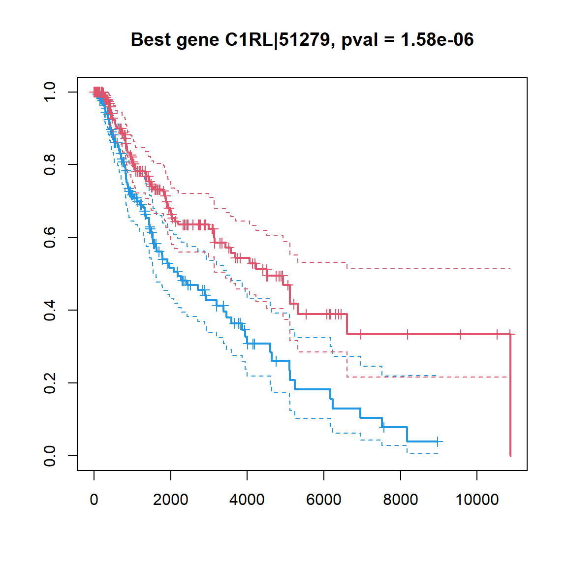
## lets combine genes
score = double(ncol(X))
ip=1
for (ip in 1:ncol(X)){
    score[ip] = sum(Res$LHR[isig] * X[isig,ip])
}

mod = coxph(Sur~score)
summary(mod)
## Call:
## coxph(formula = Sur ~ score)
##
## n= 463, number of events= 154
## (10 observations deleted due to missingness)
##
## coef exp(coef) se(coef) z Pr(>|z|)
## score 0.031922 1.032437 0.004321 7.389 1.48e-13 ***
## ---
## Signif. codes: 0 '***' 0.001 '**' 0.01 '*' 0.05 '.' 0.1 ' ' 1
##
## exp(coef) exp(-coef) lower .95 upper .95
## score 1.032 0.9686 1.024 1.041
##
## Concordance= 0.682 (se = 0.024 )
## Likelihood ratio test= 51.05 on 1 df, p=9e-13
## Wald test = 54.59 on 1 df, p=1e-13
## Score (logrank) test = 56.33 on 1 df, p=6e-14## make a KM plot
## score -> factor
fscore = c("low","high")[1+as.integer(score>median(score))]
fscore = factor(fscore,levels=c("low","high"))
plot(survfit(Sur ~ fscore),col=c(4,2),lwd=c(2,1,1), conf.int = TRUE, mark.time=TRUE,
main=sprintf("Combined score, pval = %.2e", summary(mod)$sctest["pvalue"]))