2. Classification
Petr V. Nazarov, LIH
2024-10-28
Before we start, please install the following packages:
caTools- and build ROC-curves and calculate AUCe1071- support vector machine (SVM)randomForest- random forest (RF)
2.1. Classification by logistic regression
We can use logistic regression for classification: try
glm with family="binomial". Let’s test on
predicting mouse sex by weight.
Mice = read.table("http://edu.modas.lu/data/txt/mice.txt",header=T,sep="\t",as.is=FALSE)
str(Mice)
## 'data.frame': 790 obs. of 14 variables:
## $ ID : int 1 2 3 368 369 370 371 372 4 5 ...
## $ Strain : Factor w/ 40 levels "129S1/SvImJ",..: 1 1 1 1 1 1 1 1 1 1 ...
## $ Sex : Factor w/ 2 levels "f","m": 1 1 1 1 1 1 1 1 1 1 ...
## $ Starting.age : int 66 66 66 72 72 72 72 72 66 66 ...
## $ Ending.age : int 116 116 108 114 115 116 119 122 109 112 ...
## $ Starting.weight : num 19.3 19.1 17.9 18.3 20.2 18.8 19.4 18.3 17.2 19.7 ...
## $ Ending.weight : num 20.5 20.8 19.8 21 21.9 22.1 21.3 20.1 18.9 21.3 ...
## $ Weight.change : num 1.06 1.09 1.11 1.15 1.08 ...
## $ Bleeding.time : int 64 78 90 65 55 NA 49 73 41 129 ...
## $ Ionized.Ca.in.blood : num 1.2 1.15 1.16 1.26 1.23 1.21 1.24 1.17 1.25 1.14 ...
## $ Blood.pH : num 7.24 7.27 7.26 7.22 7.3 7.28 7.24 7.19 7.29 7.22 ...
## $ Bone.mineral.density: num 0.0605 0.0553 0.0546 0.0599 0.0623 0.0626 0.0632 0.0592 0.0513 0.0501 ...
## $ Lean.tissues.weight : num 14.5 13.9 13.8 15.4 15.6 16.4 16.6 16 14 16.3 ...
## $ Fat.weight : num 4.4 4.4 2.9 4.2 4.3 4.3 5.4 4.1 3.2 5.2 ...## let's remove animals with NA values
ikeep = apply(is.na(Mice),1,sum) == 0
## all variables except strain
mod0 = glm(Sex ~ .-Strain, data = Mice[ikeep,], family = "binomial")
summary(mod0)##
## Call:
## glm(formula = Sex ~ . - Strain, family = "binomial", data = Mice[ikeep,
## ])
##
## Coefficients:
## Estimate Std. Error z value Pr(>|z|)
## (Intercept) 7.714e+01 1.246e+01 6.189 6.07e-10 ***
## ID -7.552e-04 3.939e-04 -1.917 0.055213 .
## Starting.age 9.787e-03 2.302e-02 0.425 0.670684
## Ending.age 1.320e-02 1.717e-02 0.769 0.441899
## Starting.weight -4.338e-01 2.170e-01 -1.999 0.045574 *
## Ending.weight 6.482e-01 2.026e-01 3.199 0.001380 **
## Weight.change -1.106e+01 4.379e+00 -2.525 0.011554 *
## Bleeding.time -5.441e-04 3.645e-03 -0.149 0.881344
## Ionized.Ca.in.blood -1.748e+00 1.707e+00 -1.024 0.305788
## Blood.pH -7.996e+00 1.588e+00 -5.035 4.79e-07 ***
## Bone.mineral.density -3.026e+02 2.624e+01 -11.531 < 2e-16 ***
## Lean.tissues.weight 1.935e-01 5.064e-02 3.820 0.000133 ***
## Fat.weight -2.504e-02 4.502e-02 -0.556 0.578098
## ---
## Signif. codes: 0 '***' 0.001 '**' 0.01 '*' 0.05 '.' 0.1 ' ' 1
##
## (Dispersion parameter for binomial family taken to be 1)
##
## Null deviance: 1052.19 on 758 degrees of freedom
## Residual deviance: 639.57 on 746 degrees of freedom
## AIC: 665.57
##
## Number of Fisher Scoring iterations: 5## only significant
mod1 = glm(Sex ~ Blood.pH + Bone.mineral.density + Lean.tissues.weight + Ending.weight,
data = Mice[ikeep,], family = "binomial")
summary(mod1)##
## Call:
## glm(formula = Sex ~ Blood.pH + Bone.mineral.density + Lean.tissues.weight +
## Ending.weight, family = "binomial", data = Mice[ikeep, ])
##
## Coefficients:
## Estimate Std. Error z value Pr(>|z|)
## (Intercept) 60.30264 10.49961 5.743 9.28e-09 ***
## Blood.pH -7.49819 1.44791 -5.179 2.24e-07 ***
## Bone.mineral.density -277.92619 24.35660 -11.411 < 2e-16 ***
## Lean.tissues.weight 0.20197 0.04674 4.321 1.55e-05 ***
## Ending.weight 0.21222 0.03255 6.519 7.09e-11 ***
## ---
## Signif. codes: 0 '***' 0.001 '**' 0.01 '*' 0.05 '.' 0.1 ' ' 1
##
## (Dispersion parameter for binomial family taken to be 1)
##
## Null deviance: 1052.19 on 758 degrees of freedom
## Residual deviance: 664.25 on 754 degrees of freedom
## AIC: 674.25
##
## Number of Fisher Scoring iterations: 5##load some functions for ML:
source("http://r.modas.lu/LibML.r")## [1] "----------------------------------------------------------------"
## [1] "libML: Machine learning library"
## [1] "Needed:"
## [1] "randomForest" "e1071"
## [1] "Absent:"
## character(0)##predict values (this is not informative! We work on training set!)
x = predict(mod1, Mice[ikeep,], type="response")
x = factor(levels(Mice$Sex)[1+as.integer(x >0.5)],levels = levels(Mice$Sex))
CM = getConfusionMatrix(Mice$Sex[ikeep],x)
print(CM)## f m
## pred.f 300 82
## pred.m 78 299cat("Accuracy =",1 - getMCError(CM),"\n")## Accuracy = 0.7891963To test classification one should use independent training and test
sets. One method - n-fold crossvalidation. We will use
warp-up from LibML.r
Y = Mice[ikeep,"Sex"]
X = Mice[ikeep,c("Blood.pH","Bone.mineral.density", "Lean.tissues.weight", "Ending.weight")]

res = runCrossValidation(X,Y,method = "glm")
str(res)
## List of 14
## $ method : chr "glm"
## $ nfold : num 5
## $ ntry : num 10
## $ error : num 0.215
## $ accuracy : num 0.785
## $ b_error : num 0.215
## $ b_accuracy : num 0.785
## $ specificity : num 0.785
## $ sensitivity : num 0.785
## $ CM : num [1:2, 1:2] 297.5 80.5 82.7 298.3
## ..- attr(*, "dimnames")=List of 2
## .. ..$ : chr [1:2] "pred.f" "pred.m"
## .. ..$ : chr [1:2] "f" "m"
## $ sd.error : num 0.00239
## $ sd.accuracy : num 0.00239
## $ sd.specificity: num 0.00239
## $ sd.sensitivity: num 0.00239res$CM## f m
## pred.f 297.5 82.7
## pred.m 80.5 298.3res$accuracy## [1] 0.78498022.2. Feature selections: ROC curve and AUC
Let’s consider iris dataset
library(caTools)
plot(iris[,-5],col = iris[,5],pch=19)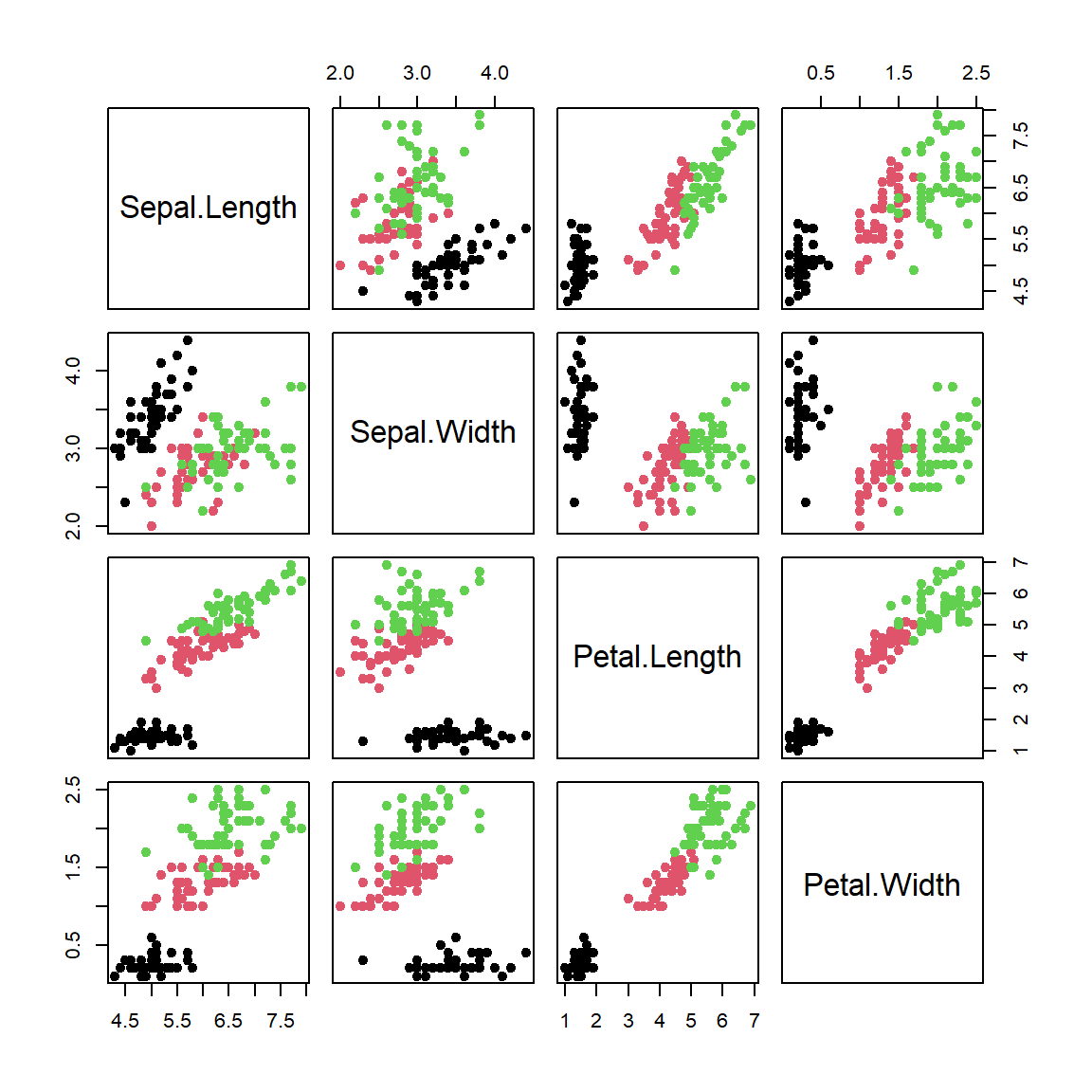
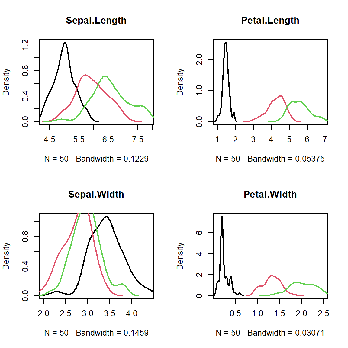
par(mfcol=c(2,2))
for (ipred in 1:4){
  plot(density(iris[as.integer(iris[,5])==1,ipred]),
       xlim=c(min(iris[,ipred]),max(iris[,ipred])),
       col=1,lwd=2,main=names(iris)[ipred])
  lines(density(iris[as.integer(iris[,5])==2,ipred]),col=2,lwd=2)
  lines(density(iris[as.integer(iris[,5])==3,ipred]),col=3,lwd=2)
}
par(mfcol=c(2,2))
colAUC(iris[,"Sepal.Length"],iris[,"Species"],plotROC=T)
## [,1]
## setosa vs. versicolor 0.9326
## setosa vs. virginica 0.9846
## versicolor vs. virginica 0.7896colAUC(iris[,"Sepal.Width"],iris[,"Species"],plotROC=T)## [,1]
## setosa vs. versicolor 0.9248
## setosa vs. virginica 0.8344
## versicolor vs. virginica 0.6636colAUC(iris[,"Petal.Length"],iris[,"Species"],plotROC=T)## [,1]
## setosa vs. versicolor 1.0000
## setosa vs. virginica 1.0000
## versicolor vs. virginica 0.9822colAUC(iris[,"Petal.Width"],iris[,"Species"],plotROC=T)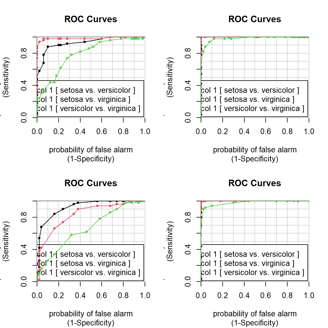
##                            [,1]
## setosa vs. versicolor    1.0000
## setosa vs. virginica     1.0000
## versicolor vs. virginica 0.9804
Another example: lung squamous cell carcinoma SCC. Here we should find the gene with the top predictive potential. Let’s use AUC.
source("http://r.modas.lu/readAMD.r")
SCC = readAMD("http://edu.modas.lu/data/txt/scc_data.txt",
              stringsAsFactors=TRUE,
              index.column=1,
sum.func="mean")str(SCC)## List of 5
## $ ncol: int 36
## $ nrow: int 17318
## $ anno:'data.frame': 17318 obs. of 2 variables:
## ..$ ID : chr [1:17318] "A1BG" "A1CF" "A2BP1" "A2LD1" ...
## ..$ Name: chr [1:17318] "NM_130786 // A1BG // alpha-1-B glycoprotein // 19q13.4 // 1 /// ENST00000263100 " "NM_138933 // A1CF // APOBEC1 complementation factor // 10q11.23 // 29974 /// NM_" "NM_018723 // A2BP1 // ataxin 2-binding protein 1 // 16p13.3 // 54715 /// NM_1458,ENST00000432184 // A2BP1 // at"| __truncated__ "NM_033110 // A2LD1 // AIG2-like domain 1 // 13q32.3 // 87769 /// ENST00000376250" ...
## $ meta:'data.frame': 36 obs. of 1 variable:
## ..$ State: Factor w/ 2 levels "cancer","normal": 1 1 1 1 1 1 1 1 1 1 ...
## $ X : num [1:17318, 1:36] 5.28 3.95 3.82 5.56 10.33 ...
## ..- attr(*, "dimnames")=List of 2
## .. ..$ : chr [1:17318] "A1BG" "A1CF" "A2BP1" "A2LD1" ...
## .. ..$ : chr [1:36] "Cancer.1" "Cancer.2" "Cancer.3" "Cancer.4" ...## colAUC gives a matrix
AUC = colAUC(t(SCC$X),SCC$meta$State,plotROC=FALSE)
## to vector
AUC = AUC[1,]
par(mfcol=c(1,2))
## plot AUC density
plot(density(AUC),main="AUC for all genes")
## how many ideal genes
sum(AUC==1)## [1] 973## let's find gene with AUC=1 and maximal logFC
logFC = apply(SCC$X[,SCC$meta$State=="cancer"],1,mean) - apply(SCC$X[,SCC$meta$State=="normal"],1,mean)
logFC[AUC<1]=0
i = which.max(abs(logFC) * AUC)
barplot(SCC$X[i,],col=c(cancer="#FF8888",normal="#8888FF")[SCC$meta$State], pch=19,main=SCC$anno[i,1],las=2,cex.names=0.5)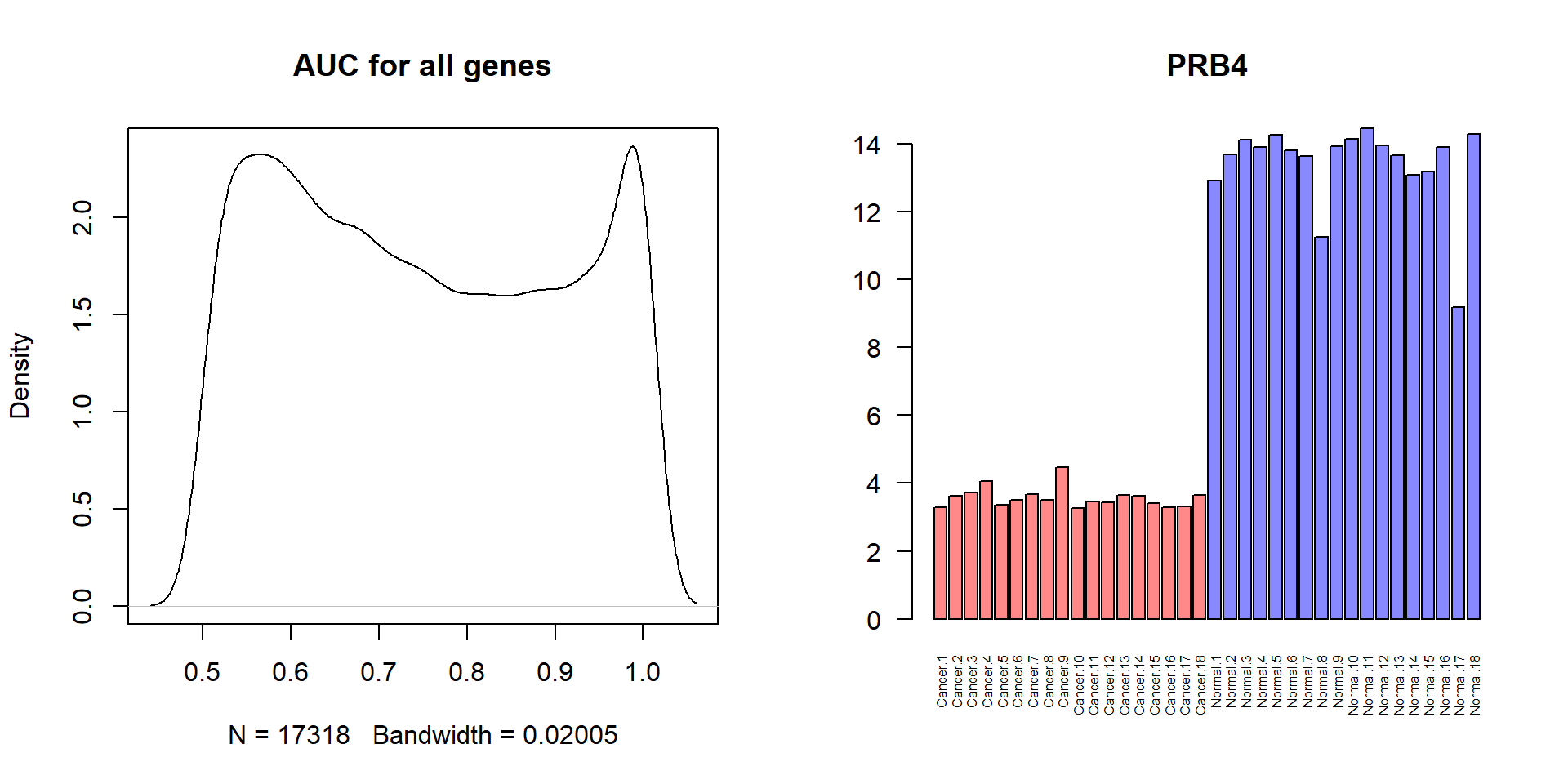
2.3. Support Vector Machine (SVM) and Random Forest (RF)
Let us build and validate classifier.
- We need to divide dataset into training and test subsets. For example trainging set - 70% of flowers and test set - 30%.
- Train SVM on training data
- Make predictions for test data and calculate misclassification error
Use svm() for SVM and randomForest for
RF.
#install.packages("e1071")
library(e1071)
library(randomForest)

itrain = sample(1:nrow(iris), 0.7 * nrow(iris) )
itest = (1:nrow(iris))[-itrain]

## SVM classifier
model1 = svm(Species ~ ., data = iris[itrain,])
## RF classifier
model2 = randomForest(Species ~ ., data = iris[itrain,])

## error on training set - should be small
pred.train = as.character(predict(model1,iris[itrain,-5]))
CM.train = getConfusionMatrix(iris[itrain,5], pred.train)
print(CM.train)
## setosa versicolor virginica
## pred.setosa 31 0 0
## pred.versicolor 0 33 2
## pred.virginica 0 0 39getAccuracy(CM.train)## [1] 0.9809524## error on test set - much more important: SVM
pred.test = as.character(predict(model1,iris[itest,-5]))
CM.test = getConfusionMatrix(iris[itest,5], pred.test)
print(CM.test)## setosa versicolor virginica
## pred.setosa 19 0 0
## pred.versicolor 0 14 0
## pred.virginica 0 3 9getAccuracy(CM.test)## [1] 0.9333333## error on test set - much more important: RF
pred.test = as.character(predict(model2,iris[itest,-5]))
CM.test = getConfusionMatrix(iris[itest,5], pred.test)
print(CM.test)## setosa versicolor virginica
## pred.setosa 19 0 0
## pred.versicolor 0 14 0
## pred.virginica 0 3 9getAccuracy(CM.test)## [1] 0.9333333Or alternatively use a warp-up to to crossvalidation:
source("http://r.modas.lu/LibML.r")## [1] "----------------------------------------------------------------"
## [1] "libML: Machine learning library"
## [1] "Needed:"
## [1] "randomForest" "e1071"
## [1] "Absent:"
## character(0)## iris example
res = runCrossValidation(iris[,-5],iris[,5],method = "svm")
res$accuracy## [1] 0.9586667## repeat: mice sex by logistic
res1 = runCrossValidation(X,Y,method = "glm")
res1$accuracy## [1] 0.784585## mice sex by support vector machines
res2 = runCrossValidation(X,Y,method = "svm")
res2$accuracy## [1] 0.7923584## mice sex by random forest
res3 = runCrossValidation(X,Y,method = "rf")
res3$accuracy## [1] 0.8113307Let’s try to predict cell types for single cell data. This cannot be solved by logistic regression (not linearly-dividable).
Panc = read.table("http://edu.modas.lu/data/txt/tsne_normpancreas.txt",sep="\t",header=TRUE,row.names=1,as.is=FALSE)
str(Panc)
## 'data.frame': 2544 obs. of 7 variables:
## $ individual : Factor w/ 8 levels "DID_scRSq01",..: 4 4 4 4 4 4 4 4 4 4 ...
## $ sex : Factor w/ 2 levels "female","male": 2 2 2 2 2 2 2 2 2 2 ...
## $ age : int 21 21 21 21 21 21 21 21 21 21 ...
## $ nreads : int 447263 412082 167913 274448 323913 419043 600361 302079 262397 227087 ...
## $ inferred.cell.type: Factor w/ 7 levels "acinar cell",..: 4 4 1 4 4 4 3 3 1 1 ...
## $ tsne1 : num 33.2 32.6 20 31.8 31 ...
## $ tsne2 : num 14 15.2 -51.6 14 16.4 ...## color - inferred cell type
col = as.integer(Panc$inferred.cell.type)+1
## shape - individual
pch=13+as.integer(Panc$individual)
## plot & legend
plot(Panc$tsne1,Panc$tsne2,pch=pch,col=col,main="tSNE with Inferred Cell Type",xlim=c(-45,50))
legend("bottomright",levels(Panc$inferred.cell.type),pch=15,col=1+(1:nlevels(Panc$inferred.cell.type)))
legend("bottomleft","shape - patient")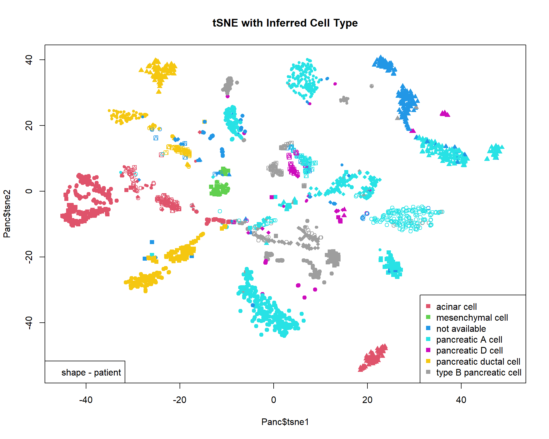
Run this yourself:
## cell type classification using support vector machines
resSVM = runCrossValidation(Panc[,c("tsne1","tsne2")],Panc$inferred.cell.type,method = "svm",echo=TRUE)
resSVM$accuracy

## cell type classification using random forest
resRF = runCrossValidation(Panc[,c("tsne1","tsne2")],Panc$inferred.cell.type,method = "rf",echo=TRUE)
resRF$accuracy

resRF$CM
Exercise 2
- Please consider breast cancer dataset of Wisconsin University
breastcancer. Please note, that the data are givein in CSV format (comma-separated values). Try building glm model to discriminate benign tumours (class=0) from malignant (class=1). Play with optimal numer of predictors. Exclude rows with NA values
glm,getMCError,predict,getConfusionMatrix,getAccuracy
- For task a - train now a classifier and report correctly calculated error. Try
glm,svm,rf. You should transform
runCrossValidationorsample,glm,svm,rf,predict,getConfusionMatrix,getMCError
| Prev Home Next |
By Petr Nazarov
|