1. Linear regression
Petr V. Nazarov, LIH
2024-10-28
1.1. Simple linear regression
Dependent variable - the variable that is being predicted or explained. Usually it is denoted by \(y\). Independent variable(s) - the variable(s) that is doing the predicting or explaining. Denoted by \(x\) or \(x_i\).
Regression model. The equation describing how y is related to x and an error term; in simple linear regression, the regression model is \(y = \beta_1 x^2 + \beta_0 + \epsilon\)
Example. Cells are grown under different temperature conditions from \(20^\circ\) to \(40^\circ\) C. A researched would like to find a dependency between T and cell number. Let us build a linear regression. And then - visualize it with confidence and predictions intervals.
Data = read.table("http://edu.modas.lu/data/txt/cells.txt", header=T,sep="\t",quote="\"")
x = Data$Temperature
y = Data$Cell.Number
mod = lm(y~x)
mod
##
## Call:
## lm(formula = y ~ x)
##
## Coefficients:
## (Intercept) x
## -190.78 15.33summary(mod)##
## Call:
## lm(formula = y ~ x)
##
## Residuals:
## Min 1Q Median 3Q Max
## -49.183 -26.190 -1.185 22.147 54.477
##
## Coefficients:
## Estimate Std. Error t value Pr(>|t|)
## (Intercept) -190.784 35.032 -5.446 2.96e-05 ***
## x 15.332 1.145 13.395 3.96e-11 ***
## ---
## Signif. codes: 0 '***' 0.001 '**' 0.01 '*' 0.05 '.' 0.1 ' ' 1
##
## Residual standard error: 31.76 on 19 degrees of freedom
## Multiple R-squared: 0.9042, Adjusted R-squared: 0.8992
## F-statistic: 179.4 on 1 and 19 DF, p-value: 3.958e-11par(mfcol=c(1,2))
# draw the data
plot(x,y,pch=19,main=sprintf("Linear model y(x) = %.1f*x + %.1f",coef(mod)[2],coef(mod)[1]))
# add the regression line and its confidence interval (95%)
lines(x, predict(mod,int = "confidence")[,1],col=2,lwd=2)
lines(x, predict(mod,int = "confidence")[,2],col=2)
lines(x, predict(mod,int = "confidence")[,3],col=2)
# add the prediction interval for the values (95%)
lines(x, predict(mod,int = "pred")[,2],col=4)
lines(x, predict(mod,int = "pred")[,3],col=4)
## draw residuals
residuals = y - (x*coef(mod)[2] + coef(mod)[1])
plot(x, residuals,pch=19,main="Residuals")
abline(h=0,col=2,lwd=2)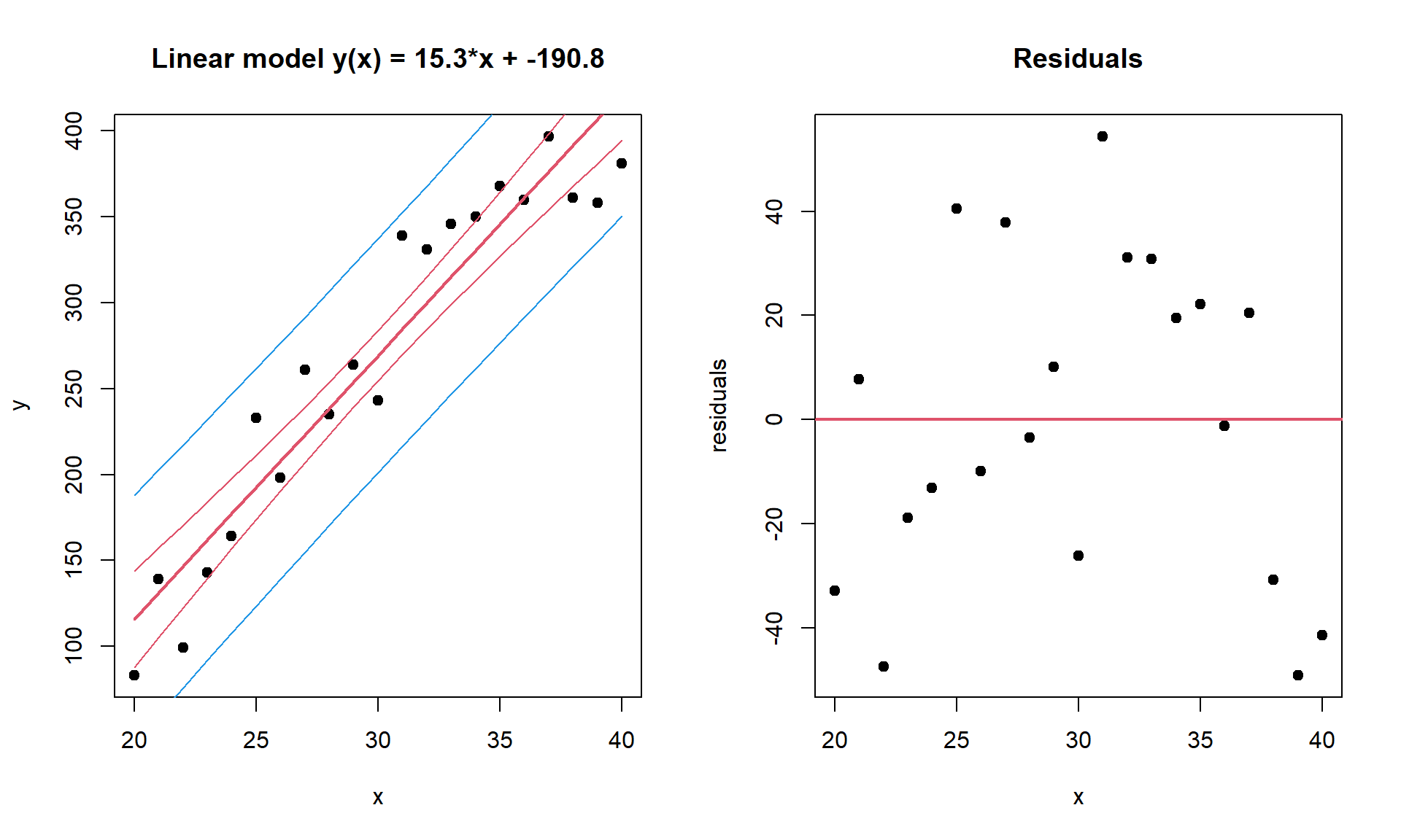
Now, let’s predict how many cells we should expect under Temperature = \(37^\circ\)C.
## confidence (where the mean will be)
predict(mod,data.frame(x=37),int = "confidence")
## fit lwr upr
## 1 376.5177 354.3436 398.6919## prediction (where the actual observation will be)
predict(mod,data.frame(x=37),int = "pred")## fit lwr upr
## 1 376.5177 306.4377 446.59783.2 Multiple linear regression
Often one variable is not enough, and we need several independent
variables to predict dependent one. Let’s consider internal
swiss dataset: standardized fertility measure and
socio-economic indicators for 47 French-speaking provinces of
Switzerland at about 1888. See ?swiss
str(swiss)## 'data.frame': 47 obs. of 6 variables:
## $ Fertility : num 80.2 83.1 92.5 85.8 76.9 76.1 83.8 92.4 82.4 82.9 ...
## $ Agriculture : num 17 45.1 39.7 36.5 43.5 35.3 70.2 67.8 53.3 45.2 ...
## $ Examination : int 15 6 5 12 17 9 16 14 12 16 ...
## $ Education : int 12 9 5 7 15 7 7 8 7 13 ...
## $ Catholic : num 9.96 84.84 93.4 33.77 5.16 ...
## $ Infant.Mortality: num 22.2 22.2 20.2 20.3 20.6 26.6 23.6 24.9 21 24.4 ...## overview of the data
#install.packages("PerformanceAnalytics")
library(PerformanceAnalytics)
chart.Correlation(swiss)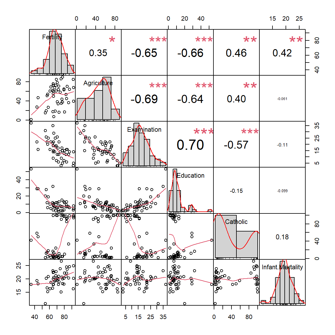
## see complete model
modAll = lm(Fertility ~ . , data = swiss)
summary(modAll)
##
## Call:
## lm(formula = Fertility ~ ., data = swiss)
##
## Residuals:
## Min 1Q Median 3Q Max
## -15.2743 -5.2617 0.5032 4.1198 15.3213
##
## Coefficients:
## Estimate Std. Error t value Pr(>|t|)
## (Intercept) 66.91518 10.70604 6.250 1.91e-07 ***
## Agriculture -0.17211 0.07030 -2.448 0.01873 *
## Examination -0.25801 0.25388 -1.016 0.31546
## Education -0.87094 0.18303 -4.758 2.43e-05 ***
## Catholic 0.10412 0.03526 2.953 0.00519 **
## Infant.Mortality 1.07705 0.38172 2.822 0.00734 **
## ---
## Signif. codes: 0 '***' 0.001 '**' 0.01 '*' 0.05 '.' 0.1 ' ' 1
##
## Residual standard error: 7.165 on 41 degrees of freedom
## Multiple R-squared: 0.7067, Adjusted R-squared: 0.671
## F-statistic: 19.76 on 5 and 41 DF, p-value: 5.594e-10## remove correlated & non-significant variable... not really correct
modSig = lm(Fertility ~ . - Examination , data = swiss)
summary(modSig)##
## Call:
## lm(formula = Fertility ~ . - Examination, data = swiss)
##
## Residuals:
## Min 1Q Median 3Q Max
## -14.6765 -6.0522 0.7514 3.1664 16.1422
##
## Coefficients:
## Estimate Std. Error t value Pr(>|t|)
## (Intercept) 62.10131 9.60489 6.466 8.49e-08 ***
## Agriculture -0.15462 0.06819 -2.267 0.02857 *
## Education -0.98026 0.14814 -6.617 5.14e-08 ***
## Catholic 0.12467 0.02889 4.315 9.50e-05 ***
## Infant.Mortality 1.07844 0.38187 2.824 0.00722 **
## ---
## Signif. codes: 0 '***' 0.001 '**' 0.01 '*' 0.05 '.' 0.1 ' ' 1
##
## Residual standard error: 7.168 on 42 degrees of freedom
## Multiple R-squared: 0.6993, Adjusted R-squared: 0.6707
## F-statistic: 24.42 on 4 and 42 DF, p-value: 1.717e-10## make simple regression using the most significant variable
mod1 = lm(Fertility ~ Education , data = swiss)
summary(mod1)##
## Call:
## lm(formula = Fertility ~ Education, data = swiss)
##
## Residuals:
## Min 1Q Median 3Q Max
## -17.036 -6.711 -1.011 9.526 19.689
##
## Coefficients:
## Estimate Std. Error t value Pr(>|t|)
## (Intercept) 79.6101 2.1041 37.836 < 2e-16 ***
## Education -0.8624 0.1448 -5.954 3.66e-07 ***
## ---
## Signif. codes: 0 '***' 0.001 '**' 0.01 '*' 0.05 '.' 0.1 ' ' 1
##
## Residual standard error: 9.446 on 45 degrees of freedom
## Multiple R-squared: 0.4406, Adjusted R-squared: 0.4282
## F-statistic: 35.45 on 1 and 45 DF, p-value: 3.659e-07## Let's remove correlated features by PCA
PC = prcomp(swiss[,-1])
swiss2 = data.frame(Fertility = swiss$Fertility, PC$x)
chart.Correlation(swiss2)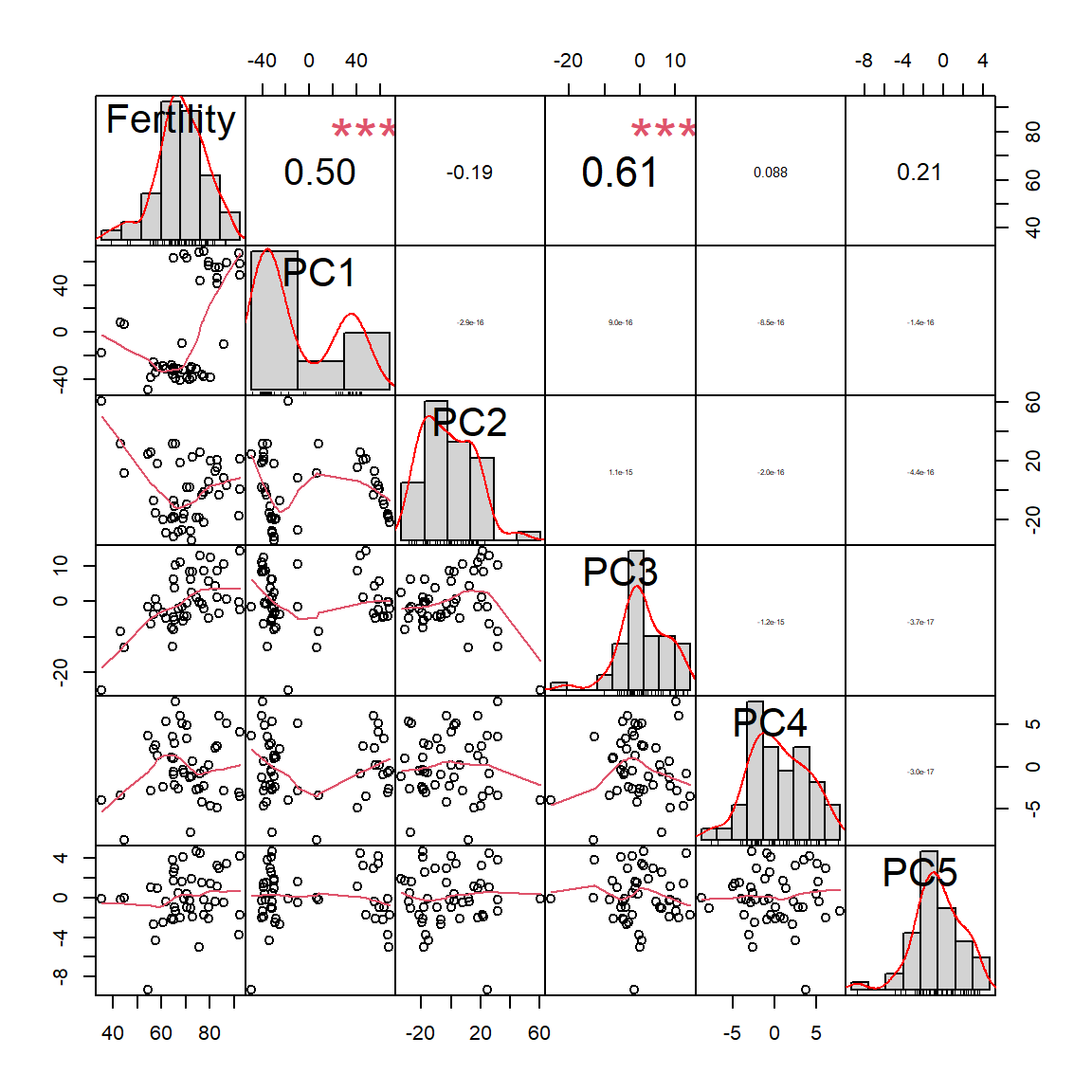
modPC = lm(Fertility ~ ., data = swiss2)
summary(modPC)
##
## Call:
## lm(formula = Fertility ~ ., data = swiss2)
##
## Residuals:
## Min 1Q Median 3Q Max
## -15.2743 -5.2617 0.5032 4.1198 15.3213
##
## Coefficients:
## Estimate Std. Error t value Pr(>|t|)
## (Intercept) 70.14255 1.04518 67.111 < 2e-16 ***
## PC1 0.14376 0.02437 5.900 6.00e-07 ***
## PC2 -0.11115 0.04930 -2.255 0.0296 *
## PC3 0.98882 0.13774 7.179 9.23e-09 ***
## PC4 -0.29483 0.28341 -1.040 0.3043
## PC5 -0.96327 0.38410 -2.508 0.0162 *
## ---
## Signif. codes: 0 '***' 0.001 '**' 0.01 '*' 0.05 '.' 0.1 ' ' 1
##
## Residual standard error: 7.165 on 41 degrees of freedom
## Multiple R-squared: 0.7067, Adjusted R-squared: 0.671
## F-statistic: 19.76 on 5 and 41 DF, p-value: 5.594e-10modPCSig = lm(Fertility ~ .-PC4, data = swiss2)
summary(modPCSig)##
## Call:
## lm(formula = Fertility ~ . - PC4, data = swiss2)
##
## Residuals:
## Min 1Q Median 3Q Max
## -16.276 -3.959 -0.651 4.519 14.416
##
## Coefficients:
## Estimate Std. Error t value Pr(>|t|)
## (Intercept) 70.14255 1.04620 67.045 < 2e-16 ***
## PC1 0.14376 0.02439 5.895 5.63e-07 ***
## PC2 -0.11115 0.04934 -2.253 0.0296 *
## PC3 0.98882 0.13788 7.172 8.26e-09 ***
## PC5 -0.96327 0.38448 -2.505 0.0162 *
## ---
## Signif. codes: 0 '***' 0.001 '**' 0.01 '*' 0.05 '.' 0.1 ' ' 1
##
## Residual standard error: 7.172 on 42 degrees of freedom
## Multiple R-squared: 0.699, Adjusted R-squared: 0.6703
## F-statistic: 24.38 on 4 and 42 DF, p-value: 1.76e-10How to choose the proper model? Several approaches:
maximizing adjusted R2
minimizing informations criteria: AIC or BIC. Choose minimal AIC/BIC
Add / remove variable and compare nested models using likelihood ratio or chi2 test.
## calculate AIC and select minimal AIC
AIC(mod1,modSig, modAll, modPC, modPCSig)
## df AIC
## mod1 3 348.4223
## modSig 6 325.2408
## modAll 7 326.0716
## modPC 7 326.0716
## modPCSig 6 325.2961BIC(mod1,modSig, modAll, modPC, modPCSig)## df BIC
## mod1 3 353.9727
## modSig 6 336.3417
## modAll 7 339.0226
## modPC 7 339.0226
## modPCSig 6 336.3970## Is fitting significantly better? Likelihood
anova(modAll,modSig)## Analysis of Variance Table
##
## Model 1: Fertility ~ Agriculture + Examination + Education + Catholic +
## Infant.Mortality
## Model 2: Fertility ~ (Agriculture + Examination + Education + Catholic +
## Infant.Mortality) - Examination
## Res.Df RSS Df Sum of Sq F Pr(>F)
## 1 41 2105.0
## 2 42 2158.1 -1 -53.027 1.0328 0.3155anova(modAll,mod1)## Analysis of Variance Table
##
## Model 1: Fertility ~ Agriculture + Examination + Education + Catholic +
## Infant.Mortality
## Model 2: Fertility ~ Education
## Res.Df RSS Df Sum of Sq F Pr(>F)
## 1 41 2105.0
## 2 45 4015.2 -4 -1910.2 9.3012 1.916e-05 ***
## ---
## Signif. codes: 0 '***' 0.001 '**' 0.01 '*' 0.05 '.' 0.1 ' ' 1## this is not very informative (use training set)
plot(swiss$Fertility, predict(modAll,swiss),xlab="Real Fertility",ylab="Predicted Fertility",pch=19)
abline(a=0,b=1,col=2,lty=2)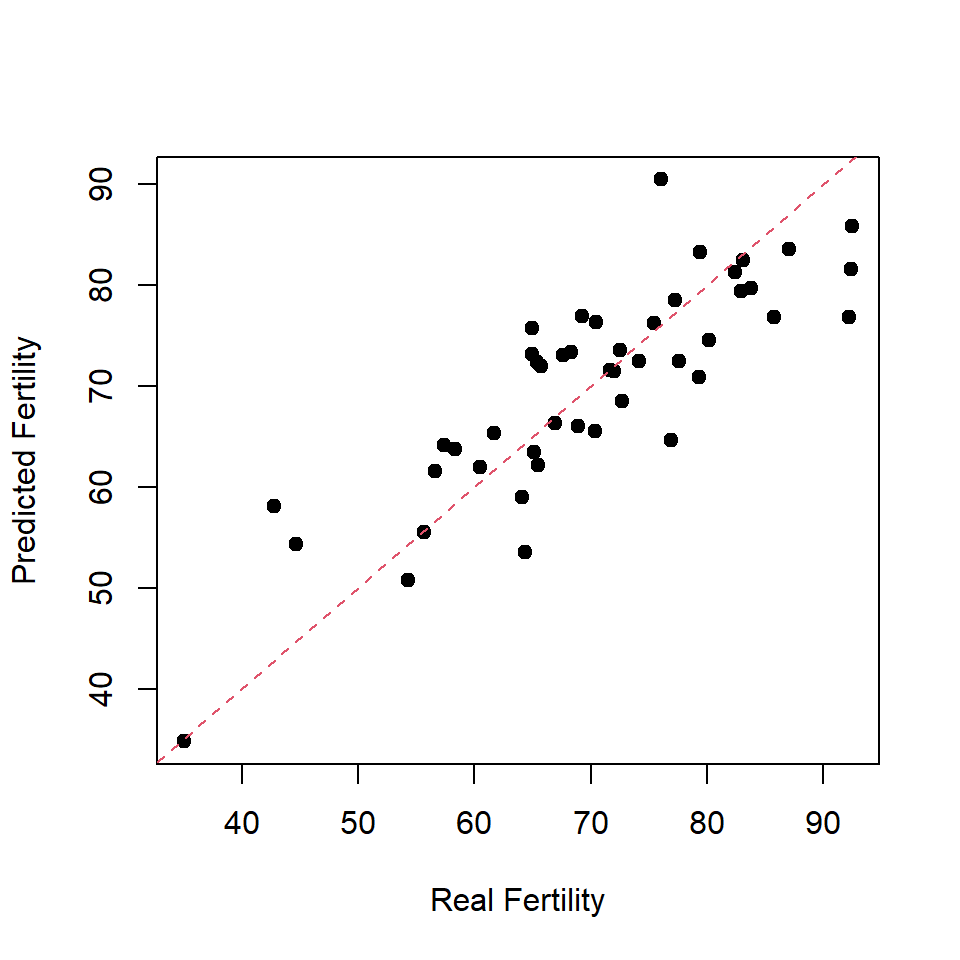
3.3 Linear regression with categorical variables
Let’s review some classical definitions regarding regression. Please note that in the literature last 15 years these terms are often mixed. Do not be surprised… :)
\[ y = function(x) \]
Univariable or “simple” model - is a model with a single independent variable (for each observation, x is a scalar)
Univariate - is a model with a single dependent variable (for each observation, y is a scalar)
Multivariable - is a model with several independent variables (for each observation, x is a vector)
Multivariate - is a model with several dependent variables (for each observation, y is a vector)
Often multivariate is used as synonym of **multivariable*. I guess because it sounds cool :)
Example: The MASS::birthwt data frame
has 189 rows and 10 columns. The data were collected at Baystate Medical
Center, Springfield, Mass, during 1986. The dataframe includes the
following parameters (slightly modified for this course):
low - indicator of birth weight less than 2.5 kg (yes/no)
age - mother’s age in years
mwt - mother’s weight in kg at last menstrual period
race - mother’s race
smoke - smoking status during pregnancy
ptl - number of previous premature labors
ht - history of hypertension
ui - presence of uterine irritability
ftv - number of physician visits during the first trimester
bwt - birth weight in grams
Let’s import the data
BWT = read.table("http://edu.modas.lu/data/txt/birthwt.txt",header=TRUE, sep="\t",comment.char="#",as.is=FALSE)
str(BWT)
## 'data.frame': 189 obs. of 10 variables:
## $ low : Factor w/ 2 levels "no","yes": 1 1 1 1 1 1 1 1 1 1 ...
## $ age : int 19 33 20 21 18 21 22 17 29 26 ...
## $ mwt : num 82.6 70.3 47.6 49 48.5 56.2 53.5 46.7 55.8 51.3 ...
## $ race : Factor w/ 3 levels "black","other",..: 1 2 3 3 3 2 3 2 3 3 ...
## $ smoke: Factor w/ 2 levels "no","yes": 1 1 2 2 2 1 1 1 2 2 ...
## $ ptl : int 0 0 0 0 0 0 0 0 0 0 ...
## $ ht : Factor w/ 2 levels "no","yes": 1 1 1 1 1 1 1 1 1 1 ...
## $ ui : Factor w/ 2 levels "no","yes": 2 1 1 2 2 1 1 1 1 1 ...
## $ ftv : int 0 3 1 2 0 0 1 1 1 0 ...
## $ bwt : int 2523 2551 2557 2594 2600 2622 2637 2637 2663 2665 ...Let’s fit simple linear regression model: \[ y = \beta_0 + \beta_1 \times x\] where y
- bwt (child birth weight), x - mwt (mother
weight)
Let’s use (for the first time) ggplots (tidy style). It is easier to
visualize regression with them. So, use
install.packages("ggplot2")
# Fit regression model
mod1 = lm(bwt ~ mwt, data = BWT)
summary(mod1)
##
## Call:
## lm(formula = bwt ~ mwt, data = BWT)
##
## Residuals:
## Min 1Q Median 3Q Max
## -2191.77 -498.28 -3.57 508.40 2075.55
##
## Coefficients:
## Estimate Std. Error t value Pr(>|t|)
## (Intercept) 2369.252 228.502 10.369 <2e-16 ***
## mwt 9.771 3.778 2.586 0.0105 *
## ---
## Signif. codes: 0 '***' 0.001 '**' 0.01 '*' 0.05 '.' 0.1 ' ' 1
##
## Residual standard error: 718.4 on 187 degrees of freedom
## Multiple R-squared: 0.03454, Adjusted R-squared: 0.02937
## F-statistic: 6.689 on 1 and 187 DF, p-value: 0.01046library(ggplot2)
p = ggplot(BWT, aes(x = mwt, y = bwt)) +
geom_point(aes(color = race, shape = smoke)) + stat_smooth(method = "lm", color = 1)
print(p)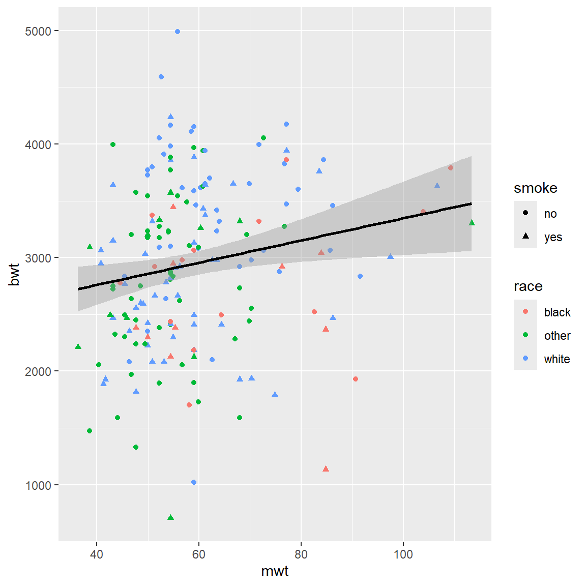
Now we will add categorical variable: smoke. So, we use
following regression:
\[ bwt = \beta_{0, smoke} + \beta_1 \times mwt\]
mod2 = lm(bwt ~ mwt + smoke, data = BWT)
summary(mod2)
##
## Call:
## lm(formula = bwt ~ mwt + smoke, data = BWT)
##
## Residuals:
## Min 1Q Median 3Q Max
## -2031.17 -445.85 29.17 521.73 1967.73
##
## Coefficients:
## Estimate Std. Error t value Pr(>|t|)
## (Intercept) 2500.872 230.860 10.833 <2e-16 ***
## mwt 9.344 3.726 2.508 0.0130 *
## smokeyes -272.005 105.591 -2.576 0.0108 *
## ---
## Signif. codes: 0 '***' 0.001 '**' 0.01 '*' 0.05 '.' 0.1 ' ' 1
##
## Residual standard error: 707.8 on 186 degrees of freedom
## Multiple R-squared: 0.0678, Adjusted R-squared: 0.05777
## F-statistic: 6.763 on 2 and 186 DF, p-value: 0.001461# Calculate smoke-specific intercepts
intercepts = c(coef(mod2)["(Intercept)"],
coef(mod2)["(Intercept)"] + coef(mod2)["smokeyes"])
# Create dataframe with regression coefficients
lines_df = data.frame(intercepts = intercepts,
slopes = rep(coef(mod2)["mwt"], 2),
smoke = levels(BWT$smoke))
qplot(x = mwt, y = bwt, color = smoke, data = BWT) +
geom_abline(aes(intercept = intercepts,
slope = slopes,
color = smoke), data = lines_df)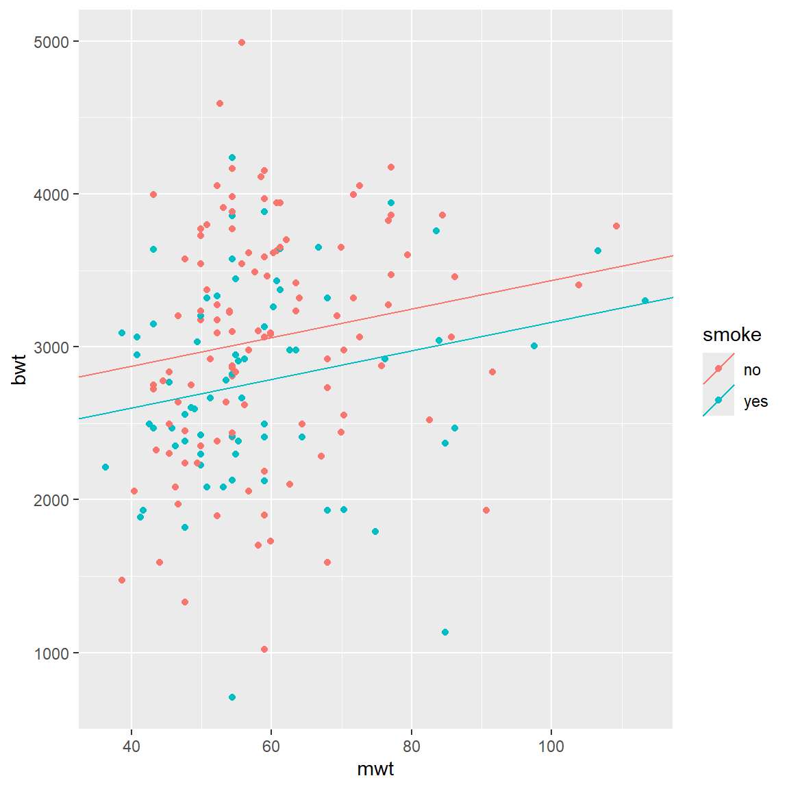
We can do the same with race:
\[ bwt = \beta_{0,race} + \beta_1 \times mwt\] Please note, how intercepts are calculated now (“race black” is considered as reference!):
mod3 = lm(bwt ~ mwt + race, data = BWT)
summary(mod3)
##
## Call:
## lm(formula = bwt ~ mwt + race, data = BWT)
##
## Residuals:
## Min 1Q Median 3Q Max
## -2095.88 -419.18 41.79 478.29 1929.45
##
## Coefficients:
## Estimate Std. Error t value Pr(>|t|)
## (Intercept) 2034.454 291.619 6.976 5.22e-11 ***
## mwt 10.289 3.859 2.667 0.00834 **
## raceother 210.684 169.079 1.246 0.21432
## racewhite 451.948 157.565 2.868 0.00461 **
## ---
## Signif. codes: 0 '***' 0.001 '**' 0.01 '*' 0.05 '.' 0.1 ' ' 1
##
## Residual standard error: 703 on 185 degrees of freedom
## Multiple R-squared: 0.08533, Adjusted R-squared: 0.0705
## F-statistic: 5.753 on 3 and 185 DF, p-value: 0.0008766# Calculate race-specific intercepts
intercepts = c(coef(mod3)["(Intercept)"],
coef(mod3)["(Intercept)"] + coef(mod3)["raceother"],
coef(mod3)["(Intercept)"] + coef(mod3)["racewhite"])
# Create dataframe with regression coefficients
lines_df = data.frame(intercepts = intercepts,
slopes = rep(coef(mod2)["mwt"], 3),
race = levels(BWT$race))
qplot(x = mwt, y = bwt, color = race, data = BWT) +
geom_abline(aes(intercept = intercepts,
slope = slopes,
color = race), data = lines_df)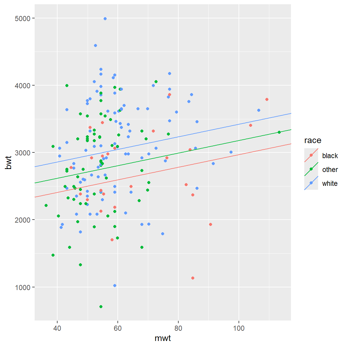
Next, we could allow slope coefficients to change as well. This will be equivalent to interactions.
\[ bwt = \beta_{0,smoke} + \beta_{1,smoke} \times mwt\]
mod4 = lm(bwt ~ mwt + smoke + mwt*smoke, data = BWT)
summary(mod4)
##
## Call:
## lm(formula = bwt ~ mwt + smoke + mwt * smoke, data = BWT)
##
## Residuals:
## Min 1Q Median 3Q Max
## -2038.59 -454.86 28.28 530.79 1976.79
##
## Coefficients:
## Estimate Std. Error t value Pr(>|t|)
## (Intercept) 2350.577 312.762 7.516 2.36e-12 ***
## mwt 11.875 5.148 2.307 0.0222 *
## smokeyes 40.929 451.209 0.091 0.9278
## mwt:smokeyes -5.330 7.471 -0.713 0.4765
## ---
## Signif. codes: 0 '***' 0.001 '**' 0.01 '*' 0.05 '.' 0.1 ' ' 1
##
## Residual standard error: 708.8 on 185 degrees of freedom
## Multiple R-squared: 0.07035, Adjusted R-squared: 0.05528
## F-statistic: 4.667 on 3 and 185 DF, p-value: 0.003617# Calculate smoke-specific intercepts
intercepts = c(coef(mod4)["(Intercept)"],
coef(mod4)["(Intercept)"] + coef(mod4)["smokeyes"])
# Calculate smoke-specific slopes
slopes = c(coef(mod4)["mwt"],
coef(mod4)["mwt"] + coef(mod4)["mwt:smokeyes"])
# Create dataframe with regression coefficients
lines_df = data.frame(intercepts = intercepts,
slopes = slopes,
smoke = levels(BWT$smoke))
qplot(x = mwt, y = bwt, color = smoke, data = BWT) +
geom_abline(aes(intercept = intercepts,
slope = slopes,
color = smoke), data = lines_df)
Same for race: \[ bwt = \beta_{0,race} +
\beta_{1,race} \times mwt\] See the loss of significance in
mod5 compared to mod3
mod5 = lm(bwt ~ mwt + race + mwt*race, data = BWT)
summary(mod5)

# Calculate smoke-specific intercepts
intercepts = c(coef(mod5)["(Intercept)"],
                coef(mod5)["(Intercept)"] + coef(mod5)["raceother"],
                coef(mod5)["(Intercept)"] + coef(mod5)["racewhite"])

# Calculate smoke-specific slopes
slopes = c(coef(mod5)["mwt"],
            coef(mod5)["mwt"] + coef(mod5)["mwt:raceother"],
            coef(mod5)["mwt"] + coef(mod5)["mwt:racewhite"])

# Create dataframe with regression coefficients
lines_df = data.frame(intercepts = intercepts,
                       slopes = slopes,
                       race = levels(BWT$race))

qplot(x = mwt, y = bwt, color = race, data = BWT) +
  geom_abline(aes(intercept = intercepts,
                  slope = slopes,
                  color = race), data = lines_df)
Check all variables and select significant:
## all variables
mod5 = lm(bwt ~ ., data = BWT[,-1])
summary(mod5)
##
## Call:
## lm(formula = bwt ~ ., data = BWT[, -1])
##
## Residuals:
## Min 1Q Median 3Q Max
## -1825.43 -435.47 55.48 473.21 1701.23
##
## Coefficients:
## Estimate Std. Error t value Pr(>|t|)
## (Intercept) 2438.861 327.262 7.452 3.77e-12 ***
## age -3.571 9.620 -0.371 0.71093
## mwt 9.609 3.826 2.511 0.01292 *
## raceother 133.531 159.396 0.838 0.40330
## racewhite 488.522 149.982 3.257 0.00135 **
## smokeyes -351.920 106.476 -3.305 0.00115 **
## ptl -48.454 101.965 -0.475 0.63522
## htyes -592.964 202.316 -2.931 0.00382 **
## uiyes -516.139 138.878 -3.716 0.00027 ***
## ftv -14.083 46.467 -0.303 0.76218
## ---
## Signif. codes: 0 '***' 0.001 '**' 0.01 '*' 0.05 '.' 0.1 ' ' 1
##
## Residual standard error: 650.3 on 179 degrees of freedom
## Multiple R-squared: 0.2428, Adjusted R-squared: 0.2047
## F-statistic: 6.377 on 9 and 179 DF, p-value: 7.849e-08## significant variables
mod6 = lm(bwt ~ mwt + race + smoke + ht + ui, data = BWT[,-1])
summary(mod6)##
## Call:
## lm(formula = bwt ~ mwt + race + smoke + ht + ui, data = BWT[,
## -1])
##
## Residuals:
## Min 1Q Median 3Q Max
## -1842.33 -432.72 67.34 459.25 1631.03
##
## Coefficients:
## Estimate Std. Error t value Pr(>|t|)
## (Intercept) 2361.538 281.653 8.385 1.36e-14 ***
## mwt 9.360 3.694 2.534 0.012121 *
## raceother 127.078 157.597 0.806 0.421094
## racewhite 475.142 145.600 3.263 0.001315 **
## smokeyes -356.207 103.444 -3.443 0.000713 ***
## htyes -585.313 199.640 -2.932 0.003802 **
## uiyes -525.592 134.667 -3.903 0.000134 ***
## ---
## Signif. codes: 0 '***' 0.001 '**' 0.01 '*' 0.05 '.' 0.1 ' ' 1
##
## Residual standard error: 645.9 on 182 degrees of freedom
## Multiple R-squared: 0.2404, Adjusted R-squared: 0.2154
## F-statistic: 9.602 on 6 and 182 DF, p-value: 3.582e-093.4. Logistic regression
Now let’s try to predict underweight in children on the same data. Logistic regression fits the following function (linear function warped in a sigmoid).
\[ y = \frac{1}{1+e^{-(\beta_0+\beta_1x_1+\beta_2x_2+...)}} = \frac{e^{\beta_0+\beta_1x_1+\beta_2x_2+...}}{1+e^{\beta_0+\beta_1x_1+\beta_2x_2+...}}\] where \(y \in [0,1]\)
Column low shows when the weight is below 2500g. Let’s
create a new variable outcome, with outcome=0 for
underweight kids and Y=1 for normal weight (it is inverted
low, but will be easier for interpretation afterwards). We
should also replace “no” with 0 and “yes” with 1 in all factors. For
factors that have more than 2 levels, use “dummy” variables :)
BWT2 = BWT ## create a new data frame
## dummy variable for race: default will be "other"
BWT2$raceblack = as.integer(BWT2$race == "black")
BWT2$racewhite = as.integer(BWT2$race == "white")
BWT2$smoke = as.integer(BWT2$smoke == "yes")
BWT2$ht = as.integer(BWT2$ht == "yes")
BWT2$ui = as.integer(BWT2$ui == "yes")
BWT2$outcome = as.integer(BWT2$low == "no")
## remove not needed columns to avoid info leackage
BWT2$low = NULL
BWT2$bwt = NULL
BWT2$race = NULL
str(BWT2)
## 'data.frame': 189 obs. of 10 variables:
## $ age : int 19 33 20 21 18 21 22 17 29 26 ...
## $ mwt : num 82.6 70.3 47.6 49 48.5 56.2 53.5 46.7 55.8 51.3 ...
## $ smoke : int 0 0 1 1 1 0 0 0 1 1 ...
## $ ptl : int 0 0 0 0 0 0 0 0 0 0 ...
## $ ht : int 0 0 0 0 0 0 0 0 0 0 ...
## $ ui : int 1 0 0 1 1 0 0 0 0 0 ...
## $ ftv : int 0 3 1 2 0 0 1 1 1 0 ...
## $ raceblack: int 1 0 0 0 0 0 0 0 0 0 ...
## $ racewhite: int 0 0 1 1 1 0 1 0 1 1 ...
## $ outcome : int 1 1 1 1 1 1 1 1 1 1 ...Now let’s see the global model (multivariable):
logmod1 = glm(outcome ~ .,family = "binomial", data = BWT2)
summary(logmod1)
##
## Call:
## glm(formula = outcome ~ ., family = "binomial", data = BWT2)
##
## Coefficients:
## Estimate Std. Error z value Pr(>|z|)
## (Intercept) -1.36253 1.10477 -1.233 0.21745
## age 0.02955 0.03703 0.798 0.42483
## mwt 0.03403 0.01526 2.230 0.02572 *
## smoke -0.93838 0.40216 -2.333 0.01963 *
## ptl -0.54362 0.34541 -1.574 0.11552
## ht -1.86375 0.69759 -2.672 0.00755 **
## ui -0.76787 0.45933 -1.672 0.09458 .
## ftv -0.06537 0.17240 -0.379 0.70455
## raceblack -0.39230 0.53768 -0.730 0.46562
## racewhite 0.88022 0.44080 1.997 0.04584 *
## ---
## Signif. codes: 0 '***' 0.001 '**' 0.01 '*' 0.05 '.' 0.1 ' ' 1
##
## (Dispersion parameter for binomial family taken to be 1)
##
## Null deviance: 234.67 on 188 degrees of freedom
## Residual deviance: 201.28 on 179 degrees of freedom
## AIC: 221.28
##
## Number of Fisher Scoring iterations: 4And only significant
logmod2 = glm(outcome ~ mwt + smoke + ht + ui + racewhite,family = "binomial", data = BWT2)
summary(logmod2)
##
## Call:
## glm(formula = outcome ~ mwt + smoke + ht + ui + racewhite, family = "binomial",
## data = BWT2)
##
## Coefficients:
## Estimate Std. Error z value Pr(>|z|)
## (Intercept) -0.90549 0.83782 -1.081 0.27980
## mwt 0.03371 0.01423 2.369 0.01786 *
## smoke -1.09082 0.38661 -2.822 0.00478 **
## ht -1.85349 0.68827 -2.693 0.00708 **
## ui -0.89284 0.44952 -1.986 0.04701 *
## racewhite 1.06467 0.38811 2.743 0.00608 **
## ---
## Signif. codes: 0 '***' 0.001 '**' 0.01 '*' 0.05 '.' 0.1 ' ' 1
##
## (Dispersion parameter for binomial family taken to be 1)
##
## Null deviance: 234.67 on 188 degrees of freedom
## Residual deviance: 204.76 on 183 degrees of freedom
## AIC: 216.76
##
## Number of Fisher Scoring iterations: 4Res = data.frame(Labels = names(coef(logmod1)))
Res$LogOdds = coef(logmod1)
Res$LogOdds1 = confint(logmod1)[,1]
Res$LogOdds2 = confint(logmod1)[,2]
(p <- ggplot(Res, aes(x = LogOdds, y = Labels)) +
geom_vline(aes(xintercept = 0), size = .25, linetype = 'dashed') +
geom_errorbarh(aes(xmax = LogOdds2, xmin = LogOdds1), linewidth = 0.5, height = 0.2, color = 'gray50') +
geom_point(size = 3.5, color = 'orange') +
theme_bw() +
theme(panel.grid.minor = element_blank()) +
scale_x_continuous(breaks = seq(-5,5,1) ) +
ylab('') +
xlab('Odds ratio (log scale)') +
ggtitle('Multivariable Model')
)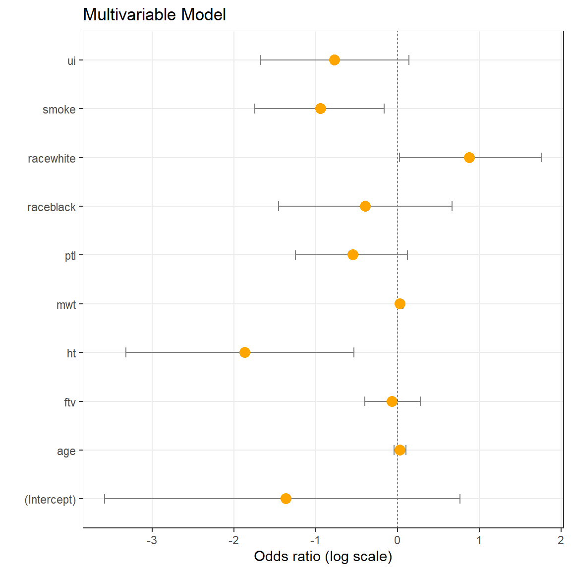
Interpretation: smoke is significantly linked to weight (lowering weight if smoke=1). racewhite positively linked to weight (increasing weight in racewhite=1), etc.
Feel free to repeat this analysis using a set of univariable models :)
Exercise 1
- A biology student wishes to determine the relationship between temperature and heart rate in leopard frog, Rana pipiens. He manipulates the temperature in \(2^\circ\) increment ranging from \(2^\circ\) to \(18^\circ\)C and records the heart rate at each interval. His data are presented in table rana.txt
- Build the model and provide the p-value for linear dependency
- Provide interval estimation for the slope of the dependency
- Estimate 95% prediction interval for heart rate at \(15^\circ\)C
lm,summary,predict,confint
- Could you estimate
Lean.tissues.weightusing other variables of Mice dataset? Please note that there are some missing datapoints which should be excluded if you are going to compare models.
lm,summary,anova,AIC
| Home Next |
By Petr Nazarov
|